Time Series

Time series models are a type of regression on a dataset with a timestamp label.

The following example creates a time series model to predict the number of forest fires in Brazil with the ‘Amazon’ dataset.

from verticapy.datasets import load_amazon
amazon = load_amazon().groupby("date", "SUM(number) AS number")
display(amazon)

	📅 date Date	123 number Integer
1	1998-01-01	0
2	1998-02-01	0
3	1998-03-01	0
4	1998-04-01	0
5	1998-05-01	0
6	1998-06-01	3551
7	1998-07-01	8066
8	1998-08-01	35549
9	1998-09-01	41968
10	1998-10-01	23495
11	1998-11-01	6804
12	1998-12-01	4448
13	1999-01-01	1081
14	1999-02-01	1284
15	1999-03-01	667
16	1999-04-01	717
17	1999-05-01	1812
18	1999-06-01	3632
19	1999-07-01	8756
20	1999-08-01	39486
21	1999-09-01	36913
22	1999-10-01	27012
23	1999-11-01	8860
24	1999-12-01	4376
25	2000-01-01	778
26	2000-02-01	561
27	2000-03-01	848
28	2000-04-01	537
29	2000-05-01	2097
30	2000-06-01	6275
31	2000-07-01	4739
32	2000-08-01	22202
33	2000-09-01	23291
34	2000-10-01	27336
35	2000-11-01	8399
36	2000-12-01	4465
37	2001-01-01	547
38	2001-02-01	1059
39	2001-03-01	1268
40	2001-04-01	1081
41	2001-05-01	2090
42	2001-06-01	8433
43	2001-07-01	6490
44	2001-08-01	31887
45	2001-09-01	39834
46	2001-10-01	31038
47	2001-11-01	15639
48	2001-12-01	6201
49	2002-01-01	1654
50	2002-02-01	1570
51	2002-03-01	1679
52	2002-04-01	1682
53	2002-05-01	3818
54	2002-06-01	10839
55	2002-07-01	13751
56	2002-08-01	57151
57	2002-09-01	55803
58	2002-10-01	47722
59	2002-11-01	28179
60	2002-12-01	11944
61	2003-01-01	5091
62	2003-02-01	2398
63	2003-03-01	2749
64	2003-04-01	2677
65	2003-05-01	1747
66	2003-06-01	6506
67	2003-07-01	11804
68	2003-08-01	43736
69	2003-09-01	76325
70	2003-10-01	43295
71	2003-11-01	23572
72	2003-12-01	15342
73	2004-01-01	2705
74	2004-02-01	1255
75	2004-03-01	2040
76	2004-04-01	1335
77	2004-05-01	3535
78	2004-06-01	14262
79	2004-07-01	23809
80	2004-08-01	49325
81	2004-09-01	83500
82	2004-10-01	40331
83	2004-11-01	30763
84	2004-12-01	17524
85	2005-01-01	4990
86	2005-02-01	2153
87	2005-03-01	1706
88	2005-04-01	1011
89	2005-05-01	3210
90	2005-06-01	5811
91	2005-07-01	15663
92	2005-08-01	51981
93	2005-09-01	76257
94	2005-10-01	49876
95	2005-11-01	21752
96	2005-12-01	6354
97	2006-01-01	3255
98	2006-02-01	1666
99	2006-03-01	1774
100	2006-04-01	792

Rows: 1-100 | Columns: 2

The feature ‘date’ tells us that we should be working with a time series model. To do predictions on time series, we use previous values called ‘lags’.

To help visualize the seasonality of forest fires, we’ll draw some autocorrelation plots.

amazon.acf(ts = "date",
           column = "number",
           p = 48)
amazon.pacf(ts = "date",
            column = "number",
            p = 48)

	value	confidence
0	1.0	0.12677953091477837
1	0.680791943478559	0.17635811053763537
2	-0.448651760602	0.19431587020757396
3	-0.056810938511524	0.1949967219550794
4	-0.214072572565421	0.19920783402950895
5	-0.132275379180003	0.20106670828355816
6	-0.209271515399161	0.20504977108289735
7	-0.22086005226401	0.20938483891715817
8	-0.115381512422639	0.21088997523164357
9	-0.0303897676702676	0.21142090542967373
10	0.195940057811936	0.21490010161856166
11	0.421096854695467	0.2288227396007685
12	0.354085600891183	0.23839868796477473
13	-0.277539454272164	0.24434402010546988
14	-0.0466619873562256	0.2450381591011353
15	-0.0252179360480865	0.2456289146925101
16	-0.0208627356674878	0.2462094909416231
17	-0.0738925038464602	0.24714597766954416
18	-0.0277152168151683	0.24775839671186392
19	-0.0570139111880927	0.2485493119105585
20	-0.0359062473532943	0.24920689325929707
21	0.0368926532844579	0.2498738171394672
22	0.183517089844233	0.25281820622976037
23	0.290406504204887	0.25925413775321304
24	0.148748898561334	0.2613732869695089
25	-0.252848551418073	0.2663277988831778
26	-0.0207691117701225	0.26698138981979946
27	0.0353140856274143	0.2676947498028233
28	-0.0921054257296545	0.26890332746753587
29	0.0154355178357686	0.2695589819239979
30	-0.0390214624263903	0.2703066482776497
31	-0.0361906130217691	0.2710449043780445
32	-0.0476484001557326	0.27185384167555554
33	-0.0190915628486309	0.2725378227507442
34	-0.0448275804550625	0.2733395375351199
35	0.311750035943525	0.28060824273716456
36	0.0433932016985829	0.2814251891164287
37	-0.115879309798946	0.28302463030064584
38	-0.0134882291090413	0.2837400527560789
39	0.0304452233355777	0.28451110093290016
40	-0.0850278455500817	0.28571394104765774
41	0.00500894018005289	0.2864362316089425
42	-0.0359016190911242	0.2872498182295229
43	-0.0515636004698935	0.288162560585811
44	-0.102742842573654	0.2896194072202406
45	-0.147438988566255	0.29184355740744294
46	-0.0890791253319279	0.2931379370389525
47	0.037269291025163	0.2939948682267675
48	-0.108829668970081	0.2955705134853683

Rows: 1-49 | Columns: 3

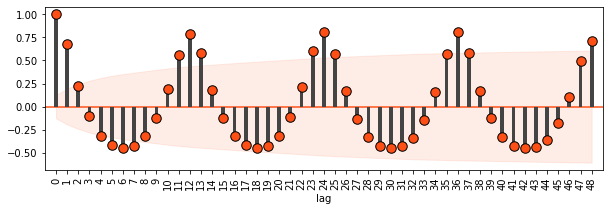
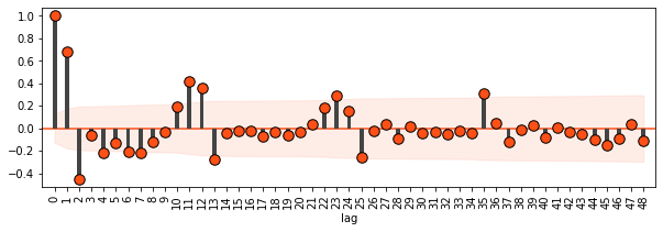
Forest fires follow a predictable, seasonal pattern, so it should be easy to predict future forest fires with past data.

VerticaPy offers several models, including a multiple time series model. For this example, let’s use a SARIMAX model.

from verticapy.learn.tsa import SARIMAX
model = SARIMAX("SARIMAX_amazon",
                p = 1,
                d = 0,
                q = 0,
                P = 4,
                D = 0,
                Q = 0,
                s = 12)
model.fit(amazon,
          y = "number",
          ts = "date")

=======
details
=======

# Coefficients

     predictor            coefficient
1    Intercept       157.796898394296
2          ar1      0.227469801171249
3         ar12      0.223437485648028
4         ar24      0.332300398258616
5         ar36      0.323432558611675
6         ar48    -0.0577341008764085
Rows: 1-6 | Columns: 2

===============
Additional Info
===============
Input Relation : (SELECT "date", "number" FROM (SELECT "date", SUM(number) AS number FROM "public"."amazon" GROUP BY 1) VERTICAPY_SUBTABLE) VERTICAPY_SUBTABLE
y : "number"
ts : "date"

Just like with other regression models, we’ll evaluate our model with the report() method.

model.report()

	value
explained_variance	0.722933514390621
max_error	62492.5846405041700760
median_absolute_error	1926.16510474475
mean_absolute_error	6244.63330879244
mean_squared_error	124238623.160803
root_mean_squared_error	11146.238072139093
r2	0.722927644647118
r2_adj	0.7149197731051271
aic	3348.6392952754804
bic	3367.2752380175016

Rows: 1-10 | Columns: 2

We can also draw our model using one-step ahead and dynamic forecasting.

model.plot(amazon,
           nlead = 150,
           dynamic = True)

<AxesSubplot:title={'center':'SARIMAX(1,0,0)(4,0,0)_12'}, xlabel='"date"'>

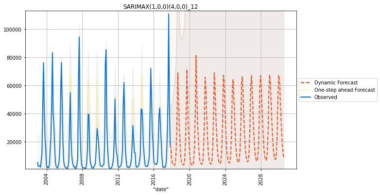
This concludes the fundamental lessons on machine learning algorithms in VerticaPy.