What Is a Range Join and Why Is It So Fast?

Last week, I was at the 2015 Conference on Innovative Data Systems Research (CIDR), held at the beautiful Asilomar Conference Grounds. The picture above shows one of the many gorgeous views you won’t see when you watch other people do PowerPoint presentations. One Vertica user at the conference said he saw a ““range join”” in a query plan, and wondered what it is and why it is so fast.

First, you need to understand what kind of queries turn into range joins. Generally, these are queries with inequality (greater than, less than, or between) predicates. For example, a map of the IPv4 address space might give details about addresses between a start and end IP for each subnet. Or, a slowly changing dimension table might, for each key, record attributes with their effective time ranges.

A rudimentary approach to handling such joins would be as follows: For each fact table row, check each dimension row to see if the range condition is true (effectively taking the Cartesian product and filtering the results). A more sophisticated, and often more efficient, approach would be to use some flavor of interval trees. However, Vertica uses a simpler approach based on sorting.

Basically, if the ranges don’t overlap very much (or at all), sorting the table by range allows sections of the table to be skipped (using a binary search or similar). For large tables, this can reduce the join time by orders of magnitude compared to ““brute force””.

Let’s take the example of a table fact, with a column fv, which we want to join to a table dim using a BETWEEN predicate against attributes dv_start and dv_end(fv>=dv_start AND fv<=dv_end). The dim table contains the following data:

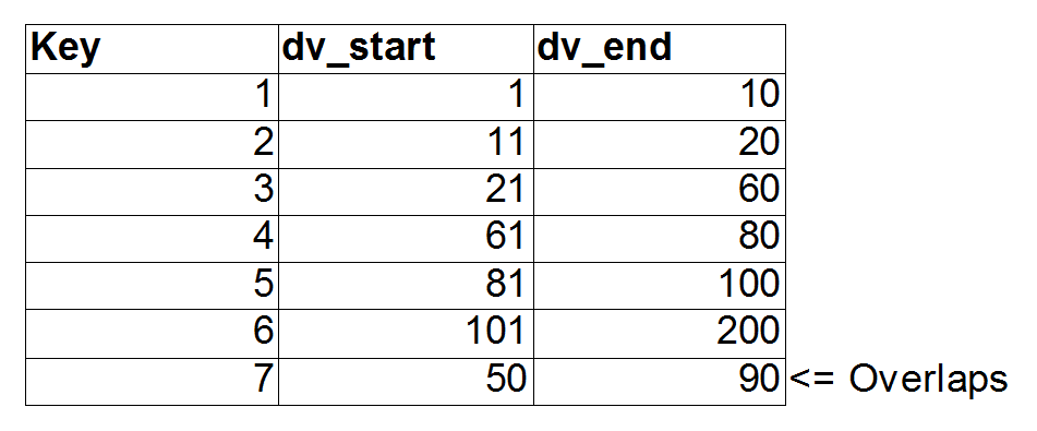
We can choose, arbitrarily, to sort the data on dv_start. This way, we can eliminate ranges that have a dv_startthat is too large to be relevant to a particular fv value. In the second figure, this is illustrated for the lookup of an fv value of 62. The left shaded red area does not need to be checked, because 62 is not greater than these dv_start values.

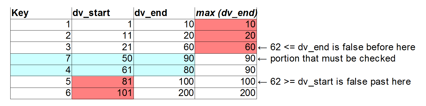
Optimizing dv_end is slightly trickier, because we have no proof that the data is sorted by dv_end (in fact, in this example, it is not). However, we can keep the largest dv_end seen in the table starting from the beginning, and search based on that. In this manner, the red area on the right can be skipped, because all of these rows have a dv_end that is not greater than 62. The part in blue, between the red areas, is then scanned to look for matches.

If you managed to follow the example, you can see our approach is simple. Yet it has helped many customers in practice. The IP subnet lookup case was the first prominent one, with a 1000x speedup. But if you got lost in this example, don’t worry… the beauty of languages like SQL is there is a community of researchers and developers who figure these things out for you. So next time you see us at a conference, don’t hesitate to ask about Vertica features. You just might see a blog about it after.