
Scatter Plots
General
Let’s begin by importing verticapy.
import verticapy as vp
Let’s also import numpy to create a random dataset.
import numpy as np
Let’s generate a dataset using the following data.
N = 20 # Number of records
data = vp.vDataFrame({
"category": [np.random.choice(['A','B','C']) for _ in range(N)],
"x": np.random.normal(5, 1, N),
"y": np.random.normal(8, 1.5, N),
"z": np.random.normal(10, 2, N),
})
In the context of data visualization, we have the flexibility to harness multiple plotting libraries to craft a wide range of graphical representations. VerticaPy, as a versatile tool, provides support for several graphic libraries, such as Matplotlib, Highcharts, and Plotly. Each of these libraries offers unique features and capabilities, allowing us to choose the most suitable one for our specific data visualization needs.

Note
To select the desired plotting library, we simply need to use the set_option() function. VerticaPy offers the flexibility to smoothly transition between different plotting libraries. In instances where a particular graphic is not supported by the chosen library or is not supported within the VerticaPy framework, the tool will automatically generate a warning and then switch to an alternative library where the graphic can be created.
Please click on the tabs to view the various graphics generated by the different plotting libraries.
We can switch to using the plotly module.
vp.set_option("plotting_lib", "plotly")
In VerticaPy, you can generate various types of scatter plots by adjusting both the number of elements and the size of the data points (bubbles), providing you with versatile options for visualizing your data.
data.scatter(columns = ["x", "y"])
We load the VerticaPy chart extension.
%load_ext verticapy.chart
We write the SQL query using Jupyter magic cells.
%%chart -k scatter
SELECT x, y FROM :data;
data.scatter(columns = ["x", "y", "z"])
We load the VerticaPy chart extension.
%load_ext verticapy.chart
We write the SQL query using Jupyter magic cells.
%%chart -k scatter
SELECT x, y, z FROM :data;
data.scatter(columns = ["x", "y"], size = "z")
We load the VerticaPy chart extension.
%load_ext verticapy.chart
We write the SQL query using Jupyter magic cells.
%%chart -k bubble
SELECT x, y, z FROM :data;
We can switch to using the highcharts module.
vp.set_option("plotting_lib", "highcharts")
In VerticaPy, you can generate various types of scatter plots by adjusting both the number of elements and the size of the data points (bubbles), providing you with versatile options for visualizing your data.
data.scatter(columns = ["x", "y"])
We load the VerticaPy chart extension.
%load_ext verticapy.chart
We write the SQL query using Jupyter magic cells.
%%chart -k scatter
SELECT x, y FROM :data;
data.scatter(columns = ["x", "y", "z"])
We load the VerticaPy chart extension.
%load_ext verticapy.chart
We write the SQL query using Jupyter magic cells.
%%chart -k scatter
SELECT x, y, z FROM :data;
data.scatter(columns = ["x", "y"], size = "z")
We load the VerticaPy chart extension.
%load_ext verticapy.chart
We write the SQL query using Jupyter magic cells.
%%chart -k bubble
SELECT x, y, z FROM :data;
We can switch to using the matplotlib module.
vp.set_option("plotting_lib", "matplotlib")
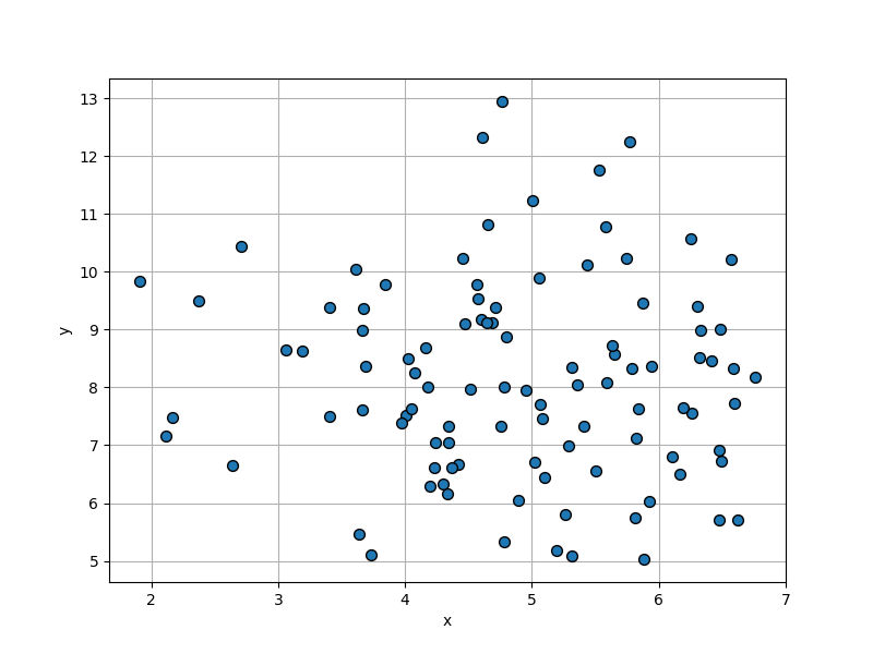
In VerticaPy, you can generate various types of scatter plots by adjusting both the number of elements and the size of the data points (bubbles), providing you with versatile options for visualizing your data.
data.scatter(columns = ["x", "y"])
Out[3]: <Axes: xlabel='x', ylabel='y'>

We load the VerticaPy chart extension.
%load_ext verticapy.chart
We write the SQL query using Jupyter magic cells.
%%chart -k scatter
SELECT x, y FROM :data;
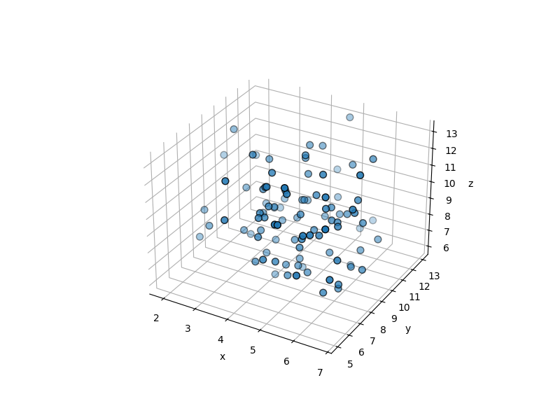
data.scatter(columns = ["x", "y", "z"])
Out[4]: <Axes3D: xlabel='x', ylabel='y', zlabel='z'>
We load the VerticaPy chart extension.
%load_ext verticapy.chart
We write the SQL query using Jupyter magic cells.
%%chart -k scatter
SELECT x, y, z FROM :data;
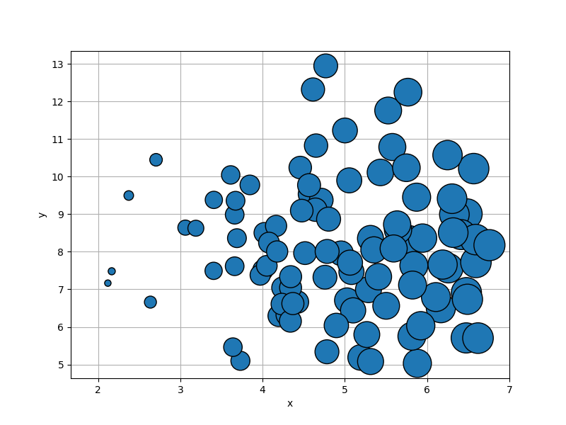
data.scatter(columns = ["x", "y"], size = "z")
Out[5]: <Axes: xlabel='x', ylabel='y'>
We load the VerticaPy chart extension.
%load_ext verticapy.chart
We write the SQL query using Jupyter magic cells.
%%chart -k bubble
SELECT x, y, z FROM :data;

PCA-Enhanced Scatter Plot for Multidimensional Data Visualization
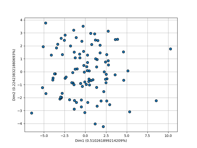
In VerticaPy, when dealing with high-dimensional data, you have the option to utilize Principal Component Analysis (PCA) for visualization purposes. VerticaPy will automatically perform the PCA transformation, and you can specify the components you wish to visualize using the “dimensions” parameter.
Note
PCA reductions are exclusively accessible through the vDataFrame object.
Using PCA components 1 & 2
data.scatter(columns = ["x", "y", "z", "t"], dimensions = (1, 2))
Using PCA components 1 & 2
data.scatter(columns = ["x", "y", "z", "t"], dimensions = (1, 2))
Using PCA components 1 & 2
data.scatter(columns = ["x", "y", "z", "t"], dimensions = (1, 2))
Out[6]: <Axes: xlabel='Dim1 (0.510261899214209%)', ylabel='Dim2 (0.224238321880693%)'>
Using Categorical and Numerical Columns for Color Representation
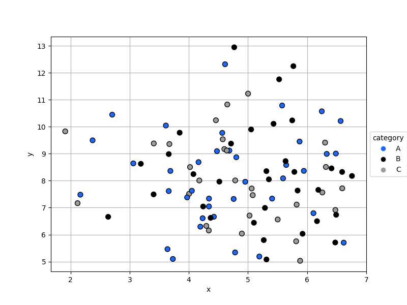
Scatter plots offer a versatile way to incorporate categorical information into your visualizations. By employing a categorical column, you can effectively represent various distinct categories within the data, with each category being visually differentiated through the use of different colors, providing a clear and intuitive representation of relationships and patterns.
Note
Enhance your scatter plots with color representation in VerticaPy. Use categorical columns to assign unique colors or employ numerical columns with a customizable colormap (cmap) for a visually rich and informative data visualization experience.
Hint
In SQL, when dealing with categorical data, it’s important to accurately represent different categories. Consider casting one of the columns as categorical using the ::VARCHAR operator for better data handling.
Using a Categorical Column
data.scatter(columns = ["x", "y"], by = "category")
%%chart -k scatter
SELECT x, y, category FROM :data;
Using a CMAP
data.scatter(columns = ["x", "y"], cmap_col = "z")
Using a Categorical Column
data.scatter(columns = ["x", "y"], by = "category")
%%chart -k scatter
SELECT x, y, category FROM :data;
Using a Categorical Column
data.scatter(columns = ["x", "y"], by = "category")
Out[7]: <Axes: xlabel='x', ylabel='y'>

%%chart -k scatter
SELECT x, y, category FROM :data;
Using a CMAP
data.scatter(columns = ["x", "y"], cmap_col = "z")
Out[8]: <Axes: xlabel='x', ylabel='y'>
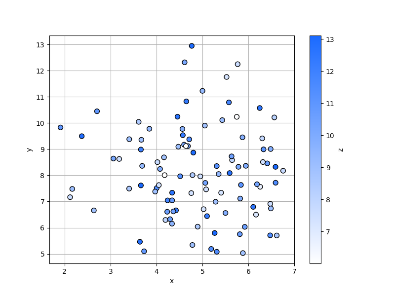
Chart Customization
VerticaPy empowers users with a high degree of flexibility when it comes to tailoring the visual aspects of their plots. This customization extends to essential elements such as color schemes, text labels, and plot sizes, as well as a wide range of other attributes that can be fine-tuned to align with specific design preferences and analytical requirements. Whether you want to make your visualizations more visually appealing or need to convey specific insights with precision, VerticaPy’s customization options enable you to craft graphics that suit your exact needs.
Hint
For SQL users who use Jupyter Magic cells, chart customization must be done in Python. They can then export the graphic using the last magic cell result.
chart = _
Now, the chart variable includes the graphic. Depending on the library you are using, you will obtain a different object.
Important
Different customization parameters are available for Plotly, Highcharts, and Matplotlib. For a comprehensive list of customization features, please consult the documentation of the respective libraries: plotly, matplotlib and highcharts.
Colors
Custom colors
fig = data.scatter(columns = ["x", "y"])
fig.update_traces(marker = dict(color="red"))
Custom colors mapping for categories
Note
You can leverage all the capabilities of the Plotly object, including functions like update_trace.
fig = data.scatter(columns = ["x", "y"], by = "category")
new_colors = ["red", "orange","green"]
for trace_index, new_color in enumerate(new_colors):
if trace_index < len(fig.data):
fig.data[trace_index].marker.color = new_color
Custom colors
data.scatter(columns = ["x", "y"], colors = ["green"])
Custom colors mapping for categories
data.scatter(columns = ["x", "y", "z"], by = "category", colors = ["red", "orange", "green"])
Custom colors
data.scatter(columns = ["x", "y"], color = ["red"])
Out[9]: <Axes: xlabel='x', ylabel='y'>

Custom colors mapping for categories
data.scatter(columns = ["x", "y", "z"], by = "category", colors = ["red", "orange", "green"])
Out[10]: <Axes3D: xlabel='x', ylabel='y', zlabel='z'>

Size
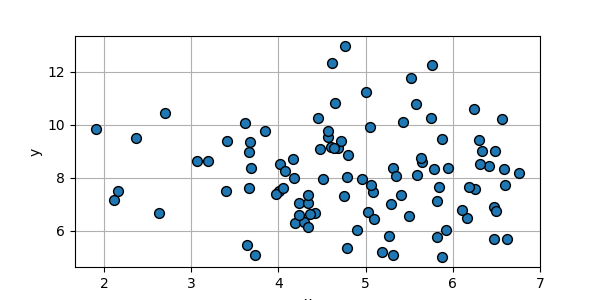
Custom Width and Height.
data.scatter(columns = ["x", "y"], width = 300, height = 300)
Custom Width and Height.
data.scatter(columns = ["x", "y"], width = 500, height = 200)
Custom Width and Height.
data.scatter(columns = ["x", "y"], width = 6, height = 3)
Out[11]: <Axes: xlabel='x', ylabel='y'>
Text
Custom Title
data.scatter(columns = ["x", "y"]).update_layout(title_text = "Custom Title")
Custom Legend Title Text
data.scatter(columns = ["x", "y"], by = 'z', legend_title_text = "Custom Legend")
Custom Axis Titles
data.scatter(columns = ["x", "y"], yaxis_title = "Custom Y-Axis Title")
Custom Title Text
data.scatter(columns = ["x", "y"], title = {"text": "Custom Title"})
Custom Axis Titles
data.scatter(columns = ["x", "y"], xAxis = {"title": {"text": "Custom X-Axis Title"}})
Custom Title Text
data.scatter(columns = ["x", "y"]).set_title("Custom Title")
Out[12]: Text(0.5, 1.0, 'Custom Title')

Custom Axis Titles
data.scatter(columns = ["x", "y"]).set_ylabel("Custom Y Axis")
Out[13]: Text(0, 0.5, 'Custom Y Axis')
