Feedback

×

• Feedback
• Was this page helpful?*
  • Yes
  • No
• Do you have any additional feedback?
  • Yes
  • No
• Additional Feedback

Africe Education

This example uses the ‘Africa Education’ dataset to predict student performance. You can can download the Jupyter Notebook of the study here.

• COUNTRY: COUNTRY ID.

• REGION: REGION ID.

• SCHOOL: SCHOOL ID.

• PUPIL: STUDENT ID.

• province: School Province.

• schoolname: School Name.

• lat: School Latitude.

• long: School Longitude.

• country_long: Country Name.

• zralocp: Student’s standardized reading score.

• zmalocp: Student’s standardized mathematics score.

• ZRALEVP: Student’s reading level.

• ZMALEVP: Student’s mathematics competency level.

• zraloct: Teacher’s standardized reading score.

• ZRALEVT: Student’s reading competency level Teacher.

• ZMALEVT: Student’s mathematics competency level Teacher.

• zsdist: School average distance from clinic, road, public, library, book shop & secondary school.

• XNUMYRS: Teacher’s years of teaching.

• numstu: Number of students at each school.

• PSEX: Student’s sex.

• PNURSERY: Student preschool.

• PENGLISH: Student speaks English at home.

• PMALIVE: Student’s biological mother alive.

• PFALIVE: Student’s biological father alive.

• PTRAVEL: Travels to school.

• PTRAVEL2: Means of transportation to school.

• PMOTHER: Mother’s education.

• PFATHER: Father’s education.

• PLIGHT: Source of lighting.

• PABSENT: Days absent.

• PREPEAT: Years repeated.

• STYPE: School type.

• SLOCAT: School location.

• SQACADEM: Academic qualifications.

• XSEX: Teacher’s sex.

• XAGE: Teacher’s age.

• XQPERMNT: Teacher’s employment status.

• XQPROFES: Teacher’s training.

• zpsibs: Student’s number of siblings.

• zpsit: Seating location.

• zpmealsc: Free school meals.

• zphmwkhl: Homework help.

• zpses: Student’s socioeconomic status.

• PAGE: Student’s Age.

• SINS2006: School inspection.

• SPUPPR04: Student dropout.

• SPUPPR06: Student cheats.

• SPUPPR07: Student uses abusive language.

• SPUPPR08: Student vandalism.

• SPUPPR09: Student theft.

• SPUPPR10: Student bullies students.

• SPUPPR11: Student bullies staff.

• SPUPPR12: Student injures staff.

• SPUPPR13: Student sexually harrasses students.

• SPUPPR14: Student sexually harrasses teachers.

• SPUPPR15: Student drug abuse.

• SPUPPR16: Student alcohol abuse.

• SPUPPR17: Student fights.

• STCHPR04: Teacher bullies students.

• STCHPR05: Teacher sexually harasses teachers.

• STCHPR06: Teacher sexually harasses students.

• STCHPR07: Teacher uses abusive language.

• STCHPR08: Teacher drug abuse.

• STCHPR09: Teacher alcohol abuse.

We will follow the data science cycle (Data Exploration - Data Preparation - Data Modeling - Model Evaluation - Model Deployment) to solve this problem.

Initialization

This example uses the following version of VerticaPy:

import verticapy as vp

vp.__version__
Out[2]: '1.1.0'

Connect to Vertica. This example uses an existing connection called VerticaDSN. For details on how to create a connection, see the Connection tutorial. You can skip the below cell if you already have an established connection.

vp.connect("VerticaDSN")

Let’s create a Virtual DataFrame of the dataset.

from verticapy.datasets import load_africa_education

africa = load_africa_education()

Warning

This example uses a sample dataset. For the full analysis, you should consider using the complete dataset.

Data Exploration and Preparation

Let’s look at the links between all the variables. Remember our goal: find a way to predict students’ final scores (zralocp & zmalocp).

africa.corr()

Some variables are useless because they are categorizations of others. For example, most scores can go from 0 to 1000, and some variables are created by mapping these variables to a reduced interval (for example: 0 to 10), so we can drop them.

africa.drop(
    [
        "ZMALEVT",
        "ZRALEVT",
        "ZRALEVP",
        "ZMALEVP",
        "COUNTRY",
        "SCHOOL",
        "PUPIL",
    ],
)

Let’s take a look at the missing values.

africa.count_percent()

	...	count	percent
"PABSENT"	...	1917.0	100.0
"zpmealsc"	...	1917.0	100.0
"PREPEAT"	...	1917.0	100.0
"lon"	...	1917.0	100.0
"zralocp"	...	1917.0	100.0
"district"	...	1917.0	100.0
"zpsit"	...	1917.0	100.0
"PNURSERY"	...	1917.0	100.0
"country_long"	...	1917.0	100.0
"PTRAVEL2"	...	1917.0	100.0
"PTRAVEL"	...	1917.0	100.0
"lat"	...	1917.0	100.0
"PLIGHT"	...	1917.0	100.0
"REGION"	...	1917.0	100.0
"PMOTHER"	...	1917.0	100.0
"PMALIVE"	...	1917.0	100.0
"PSEX"	...	1917.0	100.0
"province"	...	1917.0	100.0
"zphmwkhl"	...	1917.0	100.0
"numstu"	...	1917.0	100.0
"PFALIVE"	...	1917.0	100.0
"PENGLISH"	...	1917.0	100.0
"zpsibs"	...	1917.0	100.0
"PAGE"	...	1917.0	100.0
"schoolname"	...	1917.0	100.0
"zpses"	...	1915.0	99.896
"STYPE"	...	1914.0	99.844
"zmalocp"	...	1914.0	99.844
"SLOCAT"	...	1914.0	99.844
"XQPROFES"	...	1908.0	99.531
"XNUMYRS"	...	1908.0	99.531
"XAGE"	...	1908.0	99.531
"PFATHER"	...	1901.0	99.165
"SPUPPR16"	...	1898.0	99.009
"SPUPPR06"	...	1898.0	99.009
"SPUPPR13"	...	1898.0	99.009
"SPUPPR09"	...	1898.0	99.009
"SPUPPR10"	...	1898.0	99.009
"STCHPR08"	...	1898.0	99.009
"SUPPR17"	...	1898.0	99.009
"SPUPPR07"	...	1898.0	99.009
"SPUPPR14"	...	1898.0	99.009
"STCHPR06"	...	1898.0	99.009
"SPUPPR04"	...	1898.0	99.009
"SPUPPR11"	...	1898.0	99.009
"STCHPR07"	...	1898.0	99.009
"SQACADEM"	...	1898.0	99.009
"STCHPR04"	...	1898.0	99.009
"STCHPR09"	...	1898.0	99.009
"SPUPPR15"	...	1898.0	99.009
"SPUPPR12"	...	1898.0	99.009
"SPUPPR08"	...	1898.0	99.009
"XSEX"	...	1895.0	98.852
"SINS2006"	...	1862.0	97.131
"zsdist"	...	1838.0	95.879
"zraloct"	...	1740.0	90.767

Many values are missing for zraloct which is the teachers’ test score. We need to find a way to impute them as they represent more than 10% of the dataset. For the others that represent less than 5% of the dataset, our goal is to identify what improves student performance, so we can filter them.

We’ll use two variables to impute the teachers’ scores: TEACHER’S SEX (XSEX) and Teacher’s Training (XQPROFES).

africa["zraloct"].fillna(
    method = "avg",
    by = ["XSEX", "XQPROFES"],
)
africa.dropna()

	123 PABSENT Int 100%	...	Abc SPUPPR16 Varchar(20) 100%	Abc schoolname Varchar(16) 100%
1	9	...	NEVER	CHIKUNJA I
2	8	...	NEVER	ITISO
3	4	...	NEVER	NYAMAHAPE
4	4	...	NEVER	Omuntele Junior
5	3	...	NEVER	THABA-TELLE
6	2	...	NEVER	Bilijia Primary
7	2	...	NEVER	Ombundu Primary
8	1	...	SOMETIMES	KGABANE P/S
9	1	...	NEVER	BUHERA VILLAGE
10	1	...	NEVER	KOALI
11	1	...	NEVER	KGATLA HIGHER PR
12	1	...	NEVER	SHRI SHAMBOONATH
13	1	...	NEVER	BUHERA VILLAGE
14	0	...	SOMETIMES	Rigbo Primary Sc
15	0	...	SOMETIMES	FRANK BIGGS PRIM
16	0	...	SOMETIMES	Diyogha Junior P
17	0	...	SOMETIMES	FERDINAND BRECHE
18	0	...	SOMETIMES	FRANK BIGGS PRIM
19	0	...	SOMETIMES	MAYIBUYE PRIMARY
20	0	...	SOMETIMES	KATLEHONG GOVERN

Now that we have a clean dataset, we can use a Random Forest Regressor to understand what tends to influence the a student’s final score.

Machine Learning: Finding Clusters using lat/long

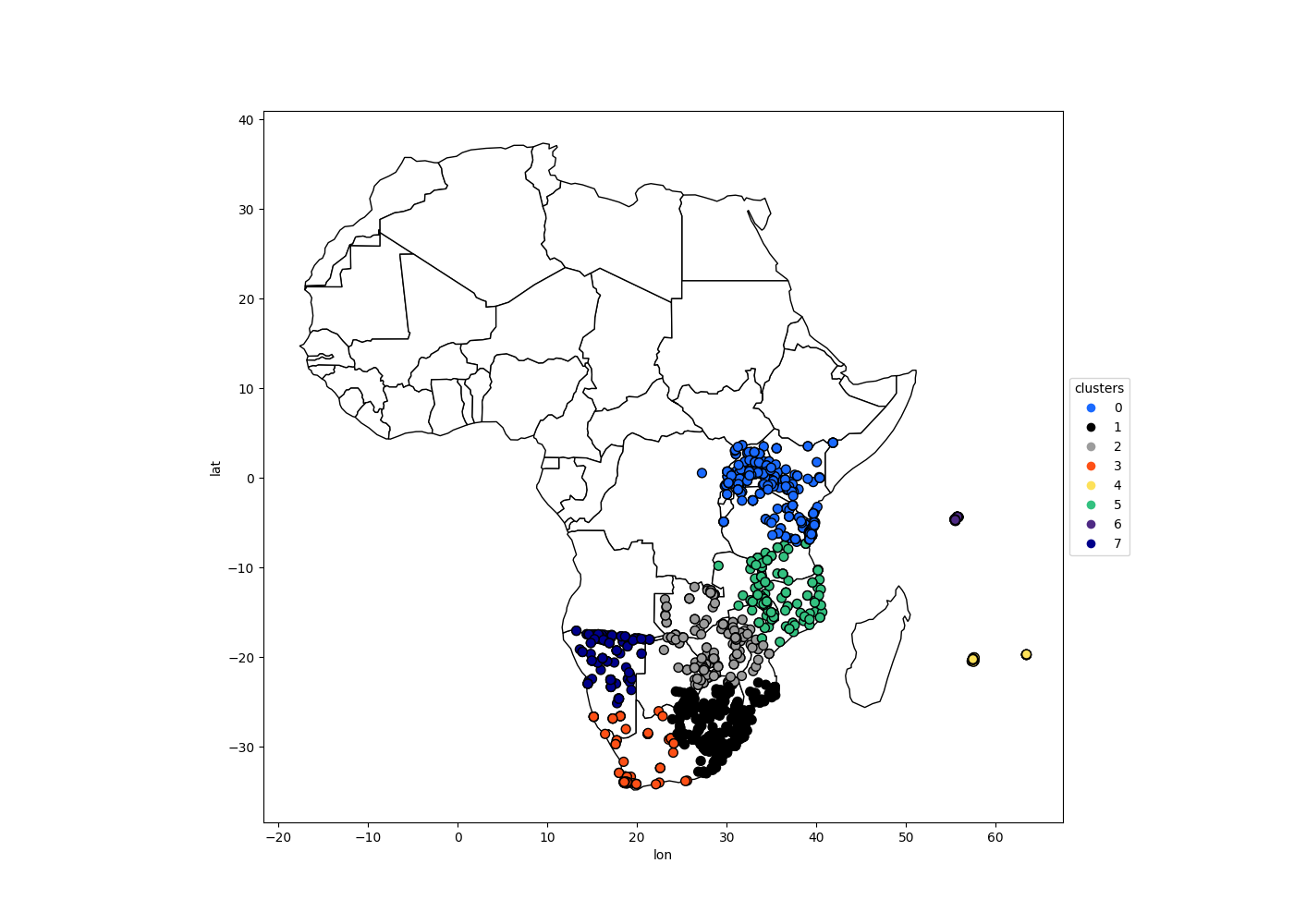
Let’s try to find some clusters between schools.

Since we have the school’s location, a natural approach might be to find school clusters based on proximity. These clusters can be used as inputs by our model.

from verticapy.machine_learning.model_selection import elbow

elbow(
    africa,
    X = ["lon", "lat"],
    n_cluster = (1, 30),
    show = True,
)

Eight seems to be a suitable number of clusters. Let’s compute a KMeans model.

from verticapy.machine_learning.vertica import KMeans

model = KMeans(n_cluster = 8)
model.fit(africa, X = ["lon", "lat"])

We can add the prediction to the vDataFrame and draw the scatter map.

# Change the plotting lib to matplotlib
vp.set_option("plotting_lib", "matplotlib")

# Adding the prediction to the vDataFrame
model.predict(africa, name = "clusters")

# Importing the World Data
from verticapy.datasets import load_world

africa_world = load_world()

# Filtering and drawing Africa
africa_world = africa_world[africa_world["continent"] == "Africa"]
ax = africa_world["geometry"].geo_plot(color = "white", edgecolor = "black",)

ax = africa_world["geometry"].geo_plot(color = "white", edgecolor = "black",)

africa.scatter(
    ["lon", "lat"],
    by = "clusters",
    ax = ax,
)

Out[6]: <Axes: xlabel='lon', ylabel='lat'>

Machine Learning: Understanding the Students’ Final Scores

A student’s math score is strongly correlated their reading score, so we can use just one of the variables for our predictions. Let’s use a cross validation to see if our variables have enough information to predict the students’ scores.

from verticapy.machine_learning.vertica import RandomForestRegressor

from verticapy.machine_learning.model_selection import cross_validate

predictors = africa.get_columns(
    exclude_columns = [
        "zralocp",
        "zmalocp",
        "lat",
        "lon",
        "schoolname",
    ],
)


response = "zralocp"

model = RandomForestRegressor(
    n_estimators = 40,
    max_depth = 20,
    min_samples_leaf = 4,
    nbins = 20,
    sample = 0.7,
)


cross_validate(
    model,
    africa,
    X = predictors,
    y = response,
)

Out[12]: 
None        ...                  bic                  time  
1-fold      ...     5701.75713930163     45.90653991699219  
2-fold      ...     5662.47802917688     47.05200791358948  
3-fold      ...     5641.05567060858    45.364285945892334  
avg         ...    5668.430279695697     46.10761125882467  
std         ...    25.13614979867821    0.7035261774052262  
Rows: 1-5 | Columns: 12

These scores are quite good! Let’s fit all the data and keep the most important variables.

model.fit(
    africa,
    X = predictors,
    y = response,
)

predictors = model.features_importance(show = False)["index"]

We can see here that socioeconomic status and a student’s country tend to strongly influence the students work quality. This makes sense: you would expect that having poor studying conditions (unstable government, difficulties at home, etc.) would lead to worse results. For now, let’s just consider the 20 most important variables.

Let’s do some tuning to find the best parameters for the use case. Our goal will be to optimize the median_absolute_error.

from verticapy.machine_learning.model_selection import grid_search_cv

gcv = grid_search_cv(
    model,
    {
        "min_samples_leaf": [1, 3],
        "max_leaf_nodes": [50],
        "max_depth": [5, 8],
    },
    metric = "median",
    input_relation = africa,
    X = predictors[:20],
    y = response,
)
gcv

Our model is excellent. Let’s create one for the students’ standardized reading score (zralocp).

response = "zralocp"
model_africa_rf_zralocp = RandomForestRegressor(**gcv["parameters"][0])
model_africa_rf_zralocp.fit(
    africa,
    predictors[0:20],
    response,
)
model_africa_rf_zralocp.regression_report()

	value
explained_variance	0.535041963138919
max_error	397.431855394128
median_absolute_error	43.832833134587
mean_absolute_error	54.1813703901185
mean_squared_error	4860.7211354088
root_mean_squared_error	69.7188721610497
r2	0.535040269050857
r2_adj	0.529836466801846
aic	15391.0184926947
bic	15505.5068018464

We’ll also create one for the students’ standardized mathematics score (zmalocp).

response = "zmalocp"
model_africa_rf_zmalocp = RandomForestRegressor(**gcv["parameters"][0])
model_africa_rf_zmalocp.fit(
    africa,
    predictors[0:20],
    response,
)
model_africa_rf_zmalocp.regression_report()

	value
explained_variance	0.455916393295267
max_error	522.60722910955
median_absolute_error	41.9959236103941
mean_absolute_error	54.0339227628776
mean_squared_error	5175.25650971217
root_mean_squared_error	71.9392556933429
r2	0.45591611404314
r2_adj	0.449826758856158
aic	15504.383882879
bic	15618.8721920307

Let’s look at the feature importance for each model.

model_africa_rf_zralocp.features_importance()

model_africa_rf_zmalocp.features_importance()

Feature importance between between math score and the reading score are almost identical.

We can add these predictions to the main vDataFrame.

africa = africa.select(predictors[0:23] + ["zralocp", "zmalocp"])
model_africa_rf_zralocp.predict(africa, name = "pred_zralocp")
model_africa_rf_zmalocp.predict(africa, name = "pred_zmalocp")

Let’s visualize our model. We begin by creating a bubble plot using the two scores.

vp.set_option("plotting_lib", "plotly")
africa.scatter(
    columns = ["zralocp", "zmalocp"],
    size = "zpses",
    by = "PENGLISH",
    max_nb_points = 2000,
)

Notable influences are home language and the socioeconomic status. It seems like students that both speak Engish at home often (but not all the time) and have a comfortable standard of living tend to perform the best.

Now, let’s see how a student’s nationality might affect their performance.

africa["country_long"].bar(
    method = "90%",
    of = "pred_zmalocp",
    max_cardinality = 50,
    width = 800,
)

africa["country_long"].bar(
    method = "10%",
    of = "pred_zmalocp",
    max_cardinality = 50,
    width = 800,
)

The students’ nationalities seem to have big impact. For example, Swaziland, Kenya, and Tanzanie are probably overrating the bad students (90% of the scores are greater than the average (500)) whereas some countries like Zambia, South Africa, and Malawi are underrating their students (90% of the scores are under 480). This could be related to the global education in the country: some education systems could be harder than the others. Let’s break this down by region.

africa["district"].bar(
    method = "50%",
    of = "pred_zmalocp",
    max_cardinality = 50,
    width = 1000,
)

The same applies to the regions. Let’s look at student age.

africa["PAGE"].barh(
    method = "50%",
    of = "pred_zmalocp",
    max_cardinality = 50,
)

Let’s look at the the variables PLIGHT (a student’s main lighting source) and PREPEAT (repeated years).

africa.bar(
    columns = ["PREPEAT", "PLIGHT"],
    method = "avg",
    of = "pred_zmalocp",
    width = 850,
)

We can see that students who never repeated a year and have light at home tend to do better in school than those who don’t.

Another factor in a student’s performance might be their method of transportation, so we’ll look at the “ptravel2” variable.

africa["ptravel2"].bar(
    method = "50%",
    of = "pred_zmalocp",
    width = 850,
)

We can clearly see that the more inconvenient it is to get to school, the worse students tend to perform.

Let’s look at the influence of the district.

Predictably, better teachers generally lead to better results. Let’s look at the influence of the district.

africa["district"].bar(
    method = "50%",
    of = "pred_zmalocp",
    h = 100,
)

Here, we can see that Chicualacuala has a very high median score, so we can conclude that a students’ district might impact their performance in school.

After assessing several predictors of student-performance, we can hypothesize some solutions. For example, we might suggest in investing in extracurricular activities, ensuring that students have adequate light sources at home, or improving public transportation.

Machine Learning: Finding the Best Students

To find the best students we can use each school’s ID (the SCHOOL variable) and compute the average score.

We can then order these by descending average score and note the top five students at each school.

africa = load_africa_education()

# Computing the averaged score
africa["score"] = (africa["zralocp"] + africa["zmalocp"]) / 2

# Computing the averaged student score
africa.analytic(
    func = "row_number",
    by = ["schoolname"],
    order_by = {"score": "desc"},
    name = "student_class_position",
)

# Finding the 3 best students by class
africa.case_when(
    "best",
    africa["student_class_position"] <= 5, 1,
    0,
)

# Selecting the main variables
africa = africa[
    [
        "PENGLISH",
        "PAGE",
        "zpses",
        "PREPEAT",
        "PTRAVEL2",
        "PLIGHT",
        "SLOCAT",
        "best",
        "zpmealsc",
        "PFATHER",
        "SPUPPR04",
        "PNURSERY",
    ]
]

# Getting the categories dummies for the Logistic Regression
africa.one_hot_encode(
    columns = [
        "PLIGHT",
        "PTRAVEL2",
        "PREPEAT",
        "PENGLISH",
        "SLOCAT",
        "PFATHER",
        "SPUPPR04",
        "PNURSERY",
        "zpmealsc"
    ],
    max_cardinality = 1000,
)
africa.dropna()

Let’s create a logistic regression to understand what circumstances allowed these students to perform as well as they have.

from verticapy.machine_learning.vertica import LogisticRegression

response = "best"
predictors = africa.get_columns(
    exclude_columns = [
        "PLIGHT",
        "PTRAVEL2",
        "PREPEAT",
        "PENGLISH",
        "SLOCAT",
        "PFATHER",
        "SPUPPR04",
        "PNURSERY",
        "zpmealsc",
        "best",
    ]
)
model_africa_logit_best = LogisticRegression(
    name="africa_logit_best",
    solver="BFGS",
)
model_africa_logit_best.fit(
    africa,
    predictors,
    response,
)
model_africa_logit_best.features_importance()

We can see that the best students tend to be young, speak English at home, come from a good socioeconomic background, have a father with a degree, and live relatively close to school.

Conclusion

We’ve solved our problem in a Pandas-like way, all without ever loading data into memory!