Feedback

×

• Feedback
• Was this page helpful?*
  • Yes
  • No
• Do you have any additional feedback?
  • Yes
  • No
• Additional Feedback

verticapy.machine_learning.vertica.ensemble.IsolationForest

class verticapy.machine_learning.vertica.ensemble.IsolationForest(name: str = None, overwrite_model: bool = False, n_estimators: int = 100, max_depth: int = 10, nbins: int = 32, sample: float = 0.632, col_sample_by_tree: float = 1.0)

Creates an IsolationForest object using the Vertica IFOREST algorithm.

Parameters

name: str, optional

Name of the model. The model is stored in the DB.

overwrite_model: bool, optional

If set to True, training a model with the same name as an existing model overwrites the existing model.

n_estimators: int, optional

The number of trees in the forest, an integer between 1 and 1000, inclusive.

max_depth: int, optional

Maximum depth of each tree, an integer between 1 and 100, inclusive.

nbins: int, optional

Number of bins used to find splits in each column, where more splits leads to a longer runtime but more fine-grained, possibly better splits. Must be an integer between 2 and 1000, inclusive.

sample: float, optional

The portion of the input data set that is randomly selected for training each tree, a float between 0.0 and 1.0, inclusive.

col_sample_by_tree: float, optional

float in the range (0,1] that specifies the fraction of columns (features), chosen at random, to use when building each tree.

Attributes

Many attributes are created during the fitting phase.

trees_: list of BinaryTreeAnomaly

Tree models are instances of ` BinaryTreeAnomaly, each possessing various attributes. For more detailed information, refer to the documentation for BinaryTreeAnomaly.

psy_: int

Sampling size used to compute the final score.

n_estimators_: int

The number of model estimators.

Note

All attributes can be accessed using the get_attributes() method.

Note

Several other attributes can be accessed by using the get_vertica_attributes() method.

Examples

The following examples provide a basic understanding of usage. For more detailed examples, please refer to the Machine Learning or the Examples section on the website.

Load data for machine learning

We import verticapy:

import verticapy as vp

Hint

By assigning an alias to verticapy, we mitigate the risk of code collisions with other libraries. This precaution is necessary because verticapy uses commonly known function names like “average” and “median”, which can potentially lead to naming conflicts. The use of an alias ensures that the functions from verticapy are used as intended without interfering with functions from other libraries.

For this example, we will use the winequality dataset.

import verticapy.datasets as vpd

data = vpd.load_winequality()

	123 fixed_acidity Numeric(8)	123 volatile_acidity Numeric(9)	123 citric_acid Numeric(8)	123 residual_sugar Numeric(9)	123 chlorides Float(22)	123 free_sulfur_dioxide Numeric(9)	123 total_sulfur_dioxide Numeric(9)	123 density Float(22)	123 pH Numeric(8)	123 sulphates Numeric(8)	123 alcohol Float(22)	123 quality Integer	123 good Integer	Abc color Varchar(20)
1	3.9	0.225	0.4	4.2	0.03	29.0	118.0	0.989	3.57	0.36	12.8	8	1	white
2	4.7	0.335	0.14	1.3	0.036	69.0	168.0	0.99212	3.47	0.46	10.5	5	0	white
3	4.7	0.455	0.18	1.9	0.036	33.0	106.0	0.98746	3.21	0.83	14.0	7	1	white
4	4.7	0.785	0.0	3.4	0.036	23.0	134.0	0.98981	3.53	0.92	13.8	6	0	white
5	4.9	0.345	0.34	1.0	0.068	32.0	143.0	0.99138	3.24	0.4	10.1	5	0	white
6	4.9	0.345	0.34	1.0	0.068	32.0	143.0	0.99138	3.24	0.4	10.1	5	0	white
7	4.9	0.42	0.0	2.1	0.048	16.0	42.0	0.99154	3.71	0.74	14.0	7	1	red
8	5.0	0.27	0.4	1.2	0.076	42.0	124.0	0.99204	3.32	0.47	10.1	6	0	white
9	5.0	0.31	0.0	6.4	0.046	43.0	166.0	0.994	3.3	0.63	9.9	6	0	white
10	5.0	0.4	0.5	4.3	0.046	29.0	80.0	0.9902	3.49	0.66	13.6	6	0	red
11	5.0	0.44	0.04	18.6	0.039	38.0	128.0	0.9985	3.37	0.57	10.2	6	0	white
12	5.1	0.11	0.32	1.6	0.028	12.0	90.0	0.99008	3.57	0.52	12.2	6	0	white
13	5.1	0.14	0.25	0.7	0.039	15.0	89.0	0.9919	3.22	0.43	9.2	6	0	white
14	5.1	0.165	0.22	5.7	0.047	42.0	146.0	0.9934	3.18	0.55	9.9	6	0	white
15	5.1	0.33	0.22	1.6	0.027	18.0	89.0	0.9893	3.51	0.38	12.5	7	1	white
16	5.1	0.33	0.22	1.6	0.027	18.0	89.0	0.9893	3.51	0.38	12.5	7	1	white
17	5.1	0.33	0.22	1.6	0.027	18.0	89.0	0.9893	3.51	0.38	12.5	7	1	white
18	5.1	0.39	0.21	1.7	0.027	15.0	72.0	0.9894	3.5	0.45	12.5	6	0	white
19	5.2	0.2	0.27	3.2	0.047	16.0	93.0	0.99235	3.44	0.53	10.1	7	1	white
20	5.2	0.21	0.31	1.7	0.048	17.0	61.0	0.98953	3.24	0.37	12.0	7	1	white
21	5.2	0.22	0.46	6.2	0.066	41.0	187.0	0.99362	3.19	0.42	9.73333333333333	5	0	white
22	5.2	0.31	0.2	2.4	0.027	27.0	117.0	0.98886	3.56	0.45	13.0	7	1	white
23	5.2	0.32	0.25	1.8	0.103	13.0	50.0	0.9957	3.38	0.55	9.2	5	0	red
24	5.2	0.34	0.37	6.2	0.031	42.0	133.0	0.99076	3.25	0.41	12.5	6	0	white
25	5.2	0.36	0.02	1.6	0.031	24.0	104.0	0.9896	3.44	0.35	12.2	6	0	white
26	5.2	0.365	0.08	13.5	0.041	37.0	142.0	0.997	3.46	0.39	9.9	6	0	white
27	5.2	0.48	0.04	1.6	0.054	19.0	106.0	0.9927	3.54	0.62	12.2	7	1	red
28	5.2	0.5	0.18	2.0	0.036	23.0	129.0	0.98949	3.36	0.77	13.4	7	1	white
29	5.3	0.16	0.39	1.0	0.028	40.0	101.0	0.99156	3.57	0.59	10.6	6	0	white
30	5.3	0.16	0.39	1.0	0.028	40.0	101.0	0.99156	3.57	0.59	10.6	6	0	white
31	5.3	0.165	0.24	1.1	0.051	25.0	105.0	0.9925	3.32	0.47	9.1	5	0	white
32	5.3	0.23	0.56	0.9	0.041	46.0	141.0	0.99119	3.16	0.62	9.7	5	0	white
33	5.3	0.3	0.3	1.2	0.029	25.0	93.0	0.98742	3.31	0.4	13.6	7	1	white
34	5.3	0.33	0.3	1.2	0.048	25.0	119.0	0.99045	3.32	0.62	11.3	6	0	white
35	5.3	0.36	0.27	6.3	0.028	40.0	132.0	0.99186	3.37	0.4	11.6	6	0	white
36	5.3	0.36	0.27	6.3	0.028	40.0	132.0	0.99186	3.37	0.4	11.6	6	0	white
37	5.3	0.4	0.25	3.9	0.031	45.0	130.0	0.99072	3.31	0.58	11.75	7	1	white
38	5.3	0.47	0.11	2.2	0.048	16.0	89.0	0.99182	3.54	0.88	13.6	7	1	red
39	5.3	0.47	0.11	2.2	0.048	16.0	89.0	0.99182	3.54	0.88	13.5666666666667	7	1	red
40	5.3	0.715	0.19	1.5	0.161	7.0	62.0	0.99395	3.62	0.61	11.0	5	0	red
41	5.4	0.22	0.29	1.2	0.045	69.0	152.0	0.99178	3.76	0.63	11.0	7	1	white
42	5.4	0.595	0.1	2.8	0.042	26.0	80.0	0.9932	3.36	0.38	9.3	5	0	white
43	5.4	0.74	0.09	1.7	0.089	16.0	26.0	0.99402	3.67	0.56	11.6	6	0	red
44	5.5	0.12	0.33	1.0	0.038	23.0	131.0	0.99164	3.25	0.45	9.8	5	0	white
45	5.5	0.12	0.33	1.0	0.038	23.0	131.0	0.99164	3.25	0.45	9.8	5	0	white
46	5.5	0.14	0.27	4.6	0.029	22.0	104.0	0.9949	3.34	0.44	9.0	5	0	white
47	5.5	0.14	0.27	4.6	0.029	22.0	104.0	0.9949	3.34	0.44	9.0	5	0	white
48	5.5	0.16	0.31	1.2	0.026	31.0	68.0	0.9898	3.33	0.44	11.65	6	0	white
49	5.5	0.16	0.31	1.2	0.026	31.0	68.0	0.9898	3.33	0.44	11.6333333333333	6	0	white
50	5.5	0.18	0.22	5.5	0.037	10.0	86.0	0.99156	3.46	0.44	12.2	5	0	white
51	5.5	0.24	0.45	1.7	0.046	22.0	113.0	0.99224	3.22	0.48	10.0	5	0	white
52	5.5	0.29	0.3	1.1	0.022	20.0	110.0	0.98869	3.34	0.38	12.8	7	1	white
53	5.5	0.31	0.29	3.0	0.027	16.0	102.0	0.99067	3.23	0.56	11.2	6	0	white
54	5.5	0.32	0.45	4.9	0.028	25.0	191.0	0.9922	3.51	0.49	11.5	7	1	white
55	5.5	0.35	0.35	1.1	0.045	14.0	167.0	0.992	3.34	0.68	9.9	6	0	white
56	5.5	0.375	0.38	1.7	0.036	17.0	98.0	0.99142	3.29	0.39	10.5	6	0	white
57	5.6	0.15	0.26	5.55	0.051	51.0	139.0	0.99336	3.47	0.5	11.0	6	0	white
58	5.6	0.15	0.31	5.3	0.038	8.0	79.0	0.9923	3.3	0.39	10.5	6	0	white
59	5.6	0.16	0.27	1.4	0.044	53.0	168.0	0.9918	3.28	0.37	10.1	6	0	white
60	5.6	0.175	0.29	0.8	0.043	20.0	67.0	0.99112	3.28	0.48	9.9	6	0	white
61	5.6	0.185	0.19	7.1	0.048	36.0	110.0	0.99438	3.26	0.41	9.5	6	0	white
62	5.6	0.185	0.19	7.1	0.048	36.0	110.0	0.99438	3.26	0.41	9.5	6	0	white
63	5.6	0.22	0.32	1.2	0.024	29.0	97.0	0.98823	3.2	0.46	13.05	7	1	white
64	5.6	0.26	0.18	1.4	0.034	18.0	135.0	0.99174	3.32	0.35	10.2	6	0	white
65	5.6	0.26	0.26	5.7	0.031	12.0	80.0	0.9923	3.25	0.38	10.8	5	0	white
66	5.6	0.26	0.5	11.4	0.029	25.0	93.0	0.99428	3.23	0.49	10.5	6	0	white
67	5.6	0.28	0.28	4.2	0.044	52.0	158.0	0.992	3.35	0.44	10.7	7	1	white
68	5.6	0.3	0.1	6.4	0.043	34.0	142.0	0.99382	3.14	0.48	9.8	5	0	white
69	5.6	0.35	0.14	5.0	0.046	48.0	198.0	0.9937	3.3	0.71	10.3	5	0	white
70	5.6	0.49	0.13	4.5	0.039	17.0	116.0	0.9907	3.42	0.9	13.7	7	1	white
71	5.6	0.49	0.13	4.5	0.039	17.0	116.0	0.9907	3.42	0.9	13.7	7	1	white
72	5.6	0.66	0.0	2.2	0.087	3.0	11.0	0.99378	3.71	0.63	12.8	7	1	red
73	5.6	0.66	0.0	2.2	0.087	3.0	11.0	0.99378	3.71	0.63	12.8	7	1	red
74	5.7	0.15	0.47	11.4	0.035	49.0	128.0	0.99456	3.03	0.34	10.5	8	1	white
75	5.7	0.18	0.26	2.2	0.023	21.0	95.0	0.9893	3.07	0.54	12.3	6	0	white
76	5.7	0.18	0.36	1.2	0.046	9.0	71.0	0.99199	3.7	0.68	10.9	7	1	white
77	5.7	0.2	0.3	2.5	0.046	38.0	125.0	0.99276	3.34	0.5	9.9	6	0	white
78	5.7	0.21	0.32	0.9	0.038	38.0	121.0	0.99074	3.24	0.46	10.6	6	0	white
79	5.7	0.21	0.37	4.5	0.04	58.0	140.0	0.99332	3.29	0.62	10.6	6	0	white
80	5.7	0.22	0.2	16.0	0.044	41.0	113.0	0.99862	3.22	0.46	8.9	6	0	white
81	5.7	0.22	0.2	16.0	0.044	41.0	113.0	0.99862	3.22	0.46	8.9	6	0	white
82	5.7	0.22	0.2	16.0	0.044	41.0	113.0	0.99862	3.22	0.46	8.9	6	0	white
83	5.7	0.22	0.2	16.0	0.044	41.0	113.0	0.99862	3.22	0.46	8.9	6	0	white
84	5.7	0.22	0.2	16.0	0.044	41.0	113.0	0.99862	3.22	0.46	8.9	6	0	white
85	5.7	0.22	0.29	3.5	0.04	27.0	146.0	0.98999	3.17	0.36	12.1	6	0	white
86	5.7	0.23	0.28	9.65	0.025	26.0	121.0	0.9925	3.28	0.38	11.3	6	0	white
87	5.7	0.25	0.26	12.5	0.049	52.5	106.0	0.99691	3.08	0.45	9.4	6	0	white
88	5.7	0.25	0.26	12.5	0.049	52.5	120.0	0.99691	3.08	0.45	9.4	6	0	white
89	5.7	0.25	0.27	11.5	0.04	24.0	120.0	0.99411	3.33	0.31	10.8	6	0	white
90	5.7	0.26	0.24	17.8	0.059	23.0	124.0	0.99773	3.3	0.5	10.1	5	0	white
91	5.7	0.26	0.24	17.8	0.059	23.0	124.0	0.99773	3.3	0.5	10.1	5	0	white
92	5.7	0.26	0.24	17.8	0.059	23.0	124.0	0.99773	3.3	0.5	10.1	5	0	white
93	5.7	0.27	0.32	1.2	0.046	20.0	155.0	0.9934	3.8	0.41	10.2	6	0	white
94	5.7	0.28	0.24	17.5	0.044	60.0	167.0	0.9989	3.31	0.44	9.4	5	0	white
95	5.7	0.32	0.18	1.4	0.029	26.0	104.0	0.9906	3.44	0.37	11.0	6	0	white
96	5.7	0.32	0.38	4.75	0.033	23.0	94.0	0.991	3.42	0.42	11.8	7	1	white
97	5.7	0.36	0.34	4.2	0.026	21.0	77.0	0.9907	3.41	0.45	11.9	6	0	white
98	5.8	0.14	0.15	6.1	0.042	27.0	123.0	0.99362	3.06	0.6	9.9	6	0	white
99	5.8	0.15	0.32	1.2	0.037	14.0	119.0	0.99137	3.19	0.5	10.2	6	0	white
100	5.8	0.17	0.34	1.8	0.045	96.0	170.0	0.99035	3.38	0.9	11.8	8	1	white

Rows: 1-100 | Columns: 14

Note

VerticaPy offers a wide range of sample datasets that are ideal for training and testing purposes. You can explore the full list of available datasets in the Datasets, which provides detailed information on each dataset and how to use them effectively. These datasets are invaluable resources for honing your data analysis and machine learning skills within the VerticaPy environment.

Model Initialization

First we import the IsolationForest model:

from verticapy.machine_learning.vertica import IsolationForest

Then we can create the model:

model = IsolationForest(
    n_estimators = 10,
    max_depth = 3,
    nbins = 6,
)

Hint

In verticapy 1.0.x and higher, you do not need to specify the model name, as the name is automatically assigned. If you need to re-use the model, you can fetch the model name from the model’s attributes.

Important

The model name is crucial for the model management system and versioning. It’s highly recommended to provide a name if you plan to reuse the model later.

Model Training

We can now fit the model:

model.fit(data, X = ["density", "sulphates"])


===========
call_string
===========
SELECT iforest('"public"."_verticapy_tmp_isolationforest_v_mldb_c0efb2cc979711efa8720242ac120002_"', '"public"."_verticapy_tmp_view_v_mldb_c1267262979711efa8720242ac120002_"', '"density", "sulphates"' USING PARAMETERS exclude_columns='', ntree=10, sampling_size=0.632, col_sample_by_tree=1, max_depth=3, nbins=6);

=======
details
=======
predictor|      type      
---------+----------------
 density |float or numeric
sulphates|float or numeric


===============
Additional Info
===============
       Name       |Value
------------------+-----
    tree_count    | 10  
rejected_row_count|  0  
accepted_row_count|6497 

Important

To train a model, you can directly use the vDataFrame or the name of the relation stored in the database. The test set is optional and is only used to compute the test metrics. In verticapy, we don’t work using X matrices and y vectors. Instead, we work directly with lists of predictors and the response name.

Hint

For clustering and anomaly detection, the use of predictors is optional. In such cases, all available predictors are considered, which can include solely numerical variables or a combination of numerical and categorical variables, depending on the model’s capabilities.

Prediction

Prediction is straight-forward:

model.predict(data, ["density", "sulphates"])

	123 fixed_acidity Numeric(8)	123 volatile_acidity Numeric(9)	123 citric_acid Numeric(8)	123 residual_sugar Numeric(9)	123 chlorides Float(22)	123 free_sulfur_dioxide Numeric(9)	123 total_sulfur_dioxide Numeric(9)	123 density Float(22)	123 pH Numeric(8)	123 sulphates Numeric(8)	123 alcohol Float(22)	123 quality Integer	123 good Integer	Abc color Varchar(20)	123 Integer
1	4.4	0.32	0.39	4.3	0.03	31.0	127.0	0.98904	3.46	0.36	12.8	8	1	white
2	4.4	0.46	0.1	2.8	0.024	31.0	111.0	0.98816	3.48	0.34	13.1	6	0	white
3	4.4	0.54	0.09	5.1	0.038	52.0	97.0	0.99022	3.41	0.4	12.2	7	1	white
4	4.7	0.6	0.17	2.3	0.058	17.0	106.0	0.9932	3.85	0.6	12.9	6	0	red
5	4.7	0.67	0.09	1.0	0.02	5.0	9.0	0.98722	3.3	0.34	13.6	5	0	white
6	4.8	0.33	0.0	6.5	0.028	34.0	163.0	0.9937	3.35	0.61	9.9	5	0	white
7	4.8	0.34	0.0	6.5	0.028	33.0	163.0	0.9939	3.36	0.61	9.9	6	0	white
8	4.9	0.47	0.17	1.9	0.035	60.0	148.0	0.98964	3.27	0.35	11.5	6	0	white
9	5.0	0.27	0.32	4.5	0.032	58.0	178.0	0.98956	3.45	0.31	12.6	7	1	white
10	5.0	0.27	0.32	4.5	0.032	58.0	178.0	0.98956	3.45	0.31	12.6	7	1	white
11	5.0	0.29	0.54	5.7	0.035	54.0	155.0	0.98976	3.27	0.34	12.9	8	1	white
12	5.0	0.33	0.18	4.6	0.032	40.0	124.0	0.99114	3.18	0.4	11.0	6	0	white
13	5.0	0.38	0.01	1.6	0.048	26.0	60.0	0.99084	3.7	0.75	14.0	6	0	red
14	5.0	0.55	0.14	8.3	0.032	35.0	164.0	0.9918	3.53	0.51	12.5	8	1	white
15	5.0	0.61	0.12	1.3	0.009	65.0	100.0	0.9874	3.26	0.37	13.5	5	0	white
16	5.1	0.21	0.28	1.4	0.047	48.0	148.0	0.99168	3.5	0.49	10.4	5	0	white
17	5.1	0.23	0.18	1.0	0.053	13.0	99.0	0.98956	3.22	0.39	11.5	5	0	white
18	5.1	0.25	0.36	1.3	0.035	40.0	78.0	0.9891	3.23	0.64	12.1	7	1	white
19	5.1	0.26	0.34	6.4	0.034	26.0	99.0	0.99449	3.23	0.41	9.2	6	0	white
20	5.1	0.35	0.26	6.8	0.034	36.0	120.0	0.99188	3.38	0.4	11.5	6	0	white
21	5.1	0.35	0.26	6.8	0.034	36.0	120.0	0.99188	3.38	0.4	11.5	6	0	white
22	5.1	0.35	0.26	6.8	0.034	36.0	120.0	0.99188	3.38	0.4	11.5	6	0	white
23	5.1	0.47	0.02	1.3	0.034	18.0	44.0	0.9921	3.9	0.62	12.8	6	0	red
24	5.1	0.585	0.0	1.7	0.044	14.0	86.0	0.99264	3.56	0.94	12.9	7	1	red
25	5.2	0.185	0.22	1.0	0.03	47.0	123.0	0.99218	3.55	0.44	10.15	6	0	white
26	5.2	0.24	0.45	3.8	0.027	21.0	128.0	0.992	3.55	0.49	11.2	8	1	white
27	5.2	0.24	0.45	3.8	0.027	21.0	128.0	0.992	3.55	0.49	11.2	8	1	white
28	5.2	0.28	0.29	1.1	0.028	18.0	69.0	0.99168	3.24	0.54	10.0	6	0	white
29	5.2	0.34	0.0	1.8	0.05	27.0	63.0	0.9916	3.68	0.79	14.0	6	0	red
30	5.2	0.34	0.0	1.8	0.05	27.0	63.0	0.9916	3.68	0.79	14.0	6	0	red
31	5.2	0.405	0.15	1.45	0.038	10.0	44.0	0.99125	3.52	0.4	11.6	4	0	white
32	5.2	0.6	0.07	7.0	0.044	33.0	147.0	0.9944	3.33	0.58	9.7	5	0	white
33	5.2	0.645	0.0	2.15	0.08	15.0	28.0	0.99444	3.78	0.61	12.5	6	0	red
34	5.3	0.2	0.31	3.6	0.036	22.0	91.0	0.99278	3.41	0.5	9.8	6	0	white
35	5.3	0.24	0.33	1.3	0.033	25.0	97.0	0.9906	3.59	0.38	11.0	8	1	white
36	5.3	0.31	0.38	10.5	0.031	53.0	140.0	0.99321	3.34	0.46	11.7	6	0	white
37	5.3	0.31	0.38	10.5	0.031	53.0	140.0	0.99321	3.34	0.46	11.7	6	0	white
38	5.3	0.395	0.07	1.3	0.035	26.0	102.0	0.992	3.5	0.35	10.6	6	0	white
39	5.3	0.43	0.11	1.1	0.029	6.0	51.0	0.99076	3.51	0.48	11.2	4	0	white
40	5.3	0.58	0.07	6.9	0.043	34.0	149.0	0.9944	3.34	0.57	9.7	5	0	white
41	5.3	0.585	0.07	7.1	0.044	34.0	145.0	0.9945	3.34	0.57	9.7	6	0	white
42	5.3	0.76	0.03	2.7	0.043	27.0	93.0	0.9932	3.34	0.38	9.2	5	0	white
43	5.4	0.18	0.24	4.8	0.041	30.0	113.0	0.99445	3.42	0.4	9.4	6	0	white
44	5.4	0.205	0.16	12.55	0.051	31.0	115.0	0.99564	3.4	0.38	10.8	6	0	white
45	5.4	0.255	0.33	1.2	0.051	29.0	122.0	0.99048	3.37	0.66	11.3	6	0	white
46	5.4	0.29	0.38	1.2	0.029	31.0	132.0	0.98895	3.28	0.36	12.4	6	0	white
47	5.4	0.29	0.38	1.2	0.029	31.0	132.0	0.98895	3.28	0.36	12.4	6	0	white
48	5.4	0.45	0.27	6.4	0.033	20.0	102.0	0.98944	3.22	0.27	13.4	8	1	white
49	5.4	0.5	0.13	5.0	0.028	12.0	107.0	0.99079	3.48	0.88	13.5	7	1	white
50	5.4	0.53	0.16	2.7	0.036	34.0	128.0	0.98856	3.2	0.53	13.2	8	1	white
51	5.4	0.53	0.16	2.7	0.036	34.0	128.0	0.98856	3.2	0.53	13.2	8	1	white
52	5.4	0.59	0.07	7.0	0.045	36.0	147.0	0.9944	3.34	0.57	9.7	6	0	white
53	5.5	0.16	0.26	1.5	0.032	35.0	100.0	0.99076	3.43	0.77	12.0	6	0	white
54	5.5	0.19	0.27	0.9	0.04	52.0	103.0	0.99026	3.5	0.39	11.2	5	0	white
55	5.5	0.23	0.19	2.2	0.044	39.0	161.0	0.99209	3.19	0.43	10.4	6	0	white
56	5.5	0.24	0.32	8.7	0.06	19.0	102.0	0.994	3.27	0.31	10.4	5	0	white
57	5.6	0.18	0.27	1.7	0.03	31.0	103.0	0.98892	3.35	0.37	12.9	6	0	white
58	5.6	0.18	0.29	2.3	0.04	5.0	47.0	0.99126	3.07	0.45	10.1	4	0	white
59	5.6	0.18	0.3	10.2	0.028	28.0	131.0	0.9954	3.49	0.42	10.8	7	1	white
60	5.6	0.18	0.31	1.5	0.038	16.0	84.0	0.9924	3.34	0.58	10.1	6	0	white
61	5.6	0.185	0.49	1.1	0.03	28.0	117.0	0.9918	3.55	0.45	10.3	6	0	white
62	5.6	0.19	0.26	1.4	0.03	12.0	76.0	0.9905	3.25	0.37	10.9	7	1	white
63	5.6	0.19	0.27	0.9	0.04	52.0	103.0	0.99026	3.5	0.39	11.2	5	0	white
64	5.6	0.19	0.31	2.7	0.027	11.0	100.0	0.98964	3.46	0.4	13.2	7	1	white
65	5.6	0.19	0.46	1.1	0.032	33.0	115.0	0.9909	3.36	0.5	10.4	6	0	white
66	5.6	0.2	0.66	10.2	0.043	78.0	175.0	0.9945	2.98	0.43	10.4	7	1	white
67	5.6	0.205	0.16	12.55	0.051	31.0	115.0	0.99564	3.4	0.38	10.8	6	0	white
68	5.6	0.225	0.24	9.8	0.054	59.0	140.0	0.99545	3.17	0.39	10.2	6	0	white
69	5.6	0.23	0.25	8.0	0.043	31.0	101.0	0.99429	3.19	0.42	10.4	6	0	white
70	5.6	0.23	0.29	3.1	0.023	19.0	89.0	0.99068	3.25	0.51	11.2	6	0	white
71	5.6	0.235	0.29	1.2	0.047	33.0	127.0	0.991	3.34	0.5	11.0	7	1	white
72	5.6	0.27	0.37	0.9	0.025	11.0	49.0	0.98845	3.29	0.33	13.1	6	0	white
73	5.6	0.28	0.27	3.9	0.043	52.0	158.0	0.99202	3.35	0.44	10.7	7	1	white
74	5.6	0.29	0.05	0.8	0.038	11.0	30.0	0.9924	3.36	0.35	9.2	5	0	white
75	5.6	0.295	0.2	2.2	0.049	18.0	134.0	0.99378	3.21	0.68	10.0	5	0	white
76	5.6	0.31	0.37	1.4	0.074	12.0	96.0	0.9954	3.32	0.58	9.2	5	0	red
77	5.6	0.33	0.28	1.2	0.031	33.0	97.0	0.99126	3.49	0.58	10.9	6	0	white
78	5.6	0.34	0.1	1.3	0.031	20.0	68.0	0.9906	3.36	0.51	11.2	7	1	white
79	5.6	0.34	0.25	2.5	0.046	47.0	182.0	0.99093	3.21	0.4	11.3	5	0	white
80	5.6	0.39	0.24	4.7	0.034	27.0	77.0	0.9906	3.28	0.36	12.7	5	0	white
81	5.6	0.41	0.22	7.1	0.05	44.0	154.0	0.9931	3.3	0.4	10.5	5	0	white
82	5.6	0.46	0.24	4.8	0.042	24.0	72.0	0.9908	3.29	0.37	12.6	6	0	white
83	5.6	0.5	0.09	2.3	0.049	17.0	99.0	0.9937	3.63	0.63	13.0	5	0	red
84	5.6	0.5	0.09	2.3	0.049	17.0	99.0	0.9937	3.63	0.63	13.0	5	0	red
85	5.6	0.605	0.05	2.4	0.073	19.0	25.0	0.99258	3.56	0.55	12.9	5	0	red
86	5.6	0.695	0.06	6.8	0.042	9.0	84.0	0.99432	3.44	0.44	10.2	5	0	white
87	5.7	0.135	0.3	4.6	0.042	19.0	101.0	0.9946	3.31	0.42	9.3	6	0	white
88	5.7	0.14	0.3	5.4	0.045	26.0	105.0	0.99469	3.32	0.45	9.3	5	0	white
89	5.7	0.18	0.22	4.2	0.042	25.0	111.0	0.994	3.35	0.39	9.4	5	0	white
90	5.7	0.22	0.22	16.65	0.044	39.0	110.0	0.99855	3.24	0.48	9.0	6	0	white
91	5.7	0.22	0.22	16.65	0.044	39.0	110.0	0.99855	3.24	0.48	9.0	6	0	white
92	5.7	0.22	0.22	16.65	0.044	39.0	110.0	0.99855	3.24	0.48	9.0	6	0	white
93	5.7	0.22	0.22	16.65	0.044	39.0	110.0	0.99855	3.24	0.48	9.0	6	0	white
94	5.7	0.22	0.28	1.3	0.027	26.0	101.0	0.98948	3.35	0.38	12.5	7	1	white
95	5.7	0.245	0.33	1.1	0.049	28.0	150.0	0.9927	3.13	0.42	9.3	5	0	white
96	5.7	0.25	0.21	1.5	0.044	21.0	108.0	0.99142	3.3	0.59	11.0	6	0	white
97	5.7	0.255	0.65	1.2	0.079	17.0	137.0	0.99307	3.2	0.42	9.4	5	0	white
98	5.7	0.255	0.65	1.2	0.079	17.0	137.0	0.99307	3.2	0.42	9.4	5	0	white
99	5.7	0.28	0.3	3.9	0.026	36.0	105.0	0.98963	3.26	0.58	12.75	6	0	white
100	5.7	0.31	0.29	7.3	0.05	33.0	143.0	0.99332	3.31	0.5	11.0666666666667	6	0	white

Rows: 1-100 | Columns: 15

Plots - Anomaly Detection

Plots highlighting the outliers can be easily drawn using:

model.plot()

Note

Most anomaly detection methods produce a score. In scenarios involving 2 or 3 predictors, using a bubble plot to visualize the model’s results is a straightforward approach. In such plots, the size of each bubble corresponds to the anomaly score.

Plots - Tree

Tree models can be visualized by drawing their tree plots. For more examples, check out Machine Learning - Tree Plots.

model.plot_tree()

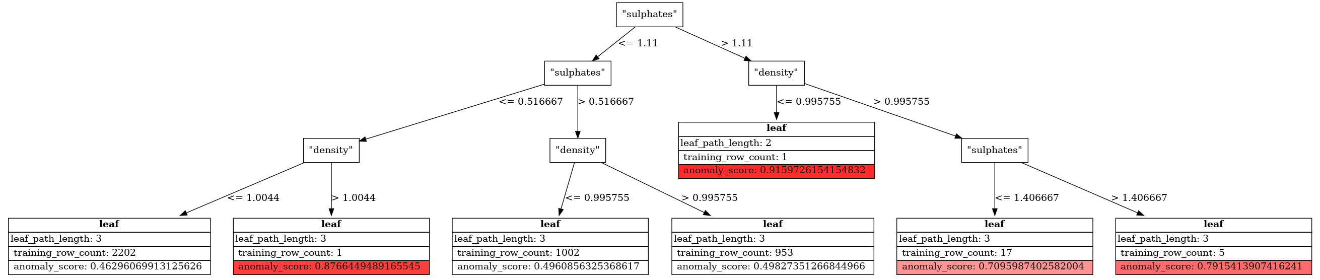
Note

The above example may not render properly in the doc because of the huge size of the tree. But it should render nicely in jupyter environment.

In order to plot graph using graphviz separately, you can extract the graphviz DOT file code as follows:

model.to_graphviz()
Out[4]: 'digraph Tree {\ngraph [bgcolor="#FFFFFFDD"];\n0 [label="\\"sulphates\\"", shape="box", style="filled", fillcolor="#FFFFFFDD", fontcolor="#000000", color="#000000"]\n0 -> 1 [label="<= 1.11", color="#000000", fontcolor="#000000"]\n0 -> 2 [label="> 1.11", color="#000000", fontcolor="#000000"]\n1 [label="\\"sulphates\\"", shape="box", style="filled", fillcolor="#FFFFFFDD", fontcolor="#000000", color="#000000"]\n1 -> 3 [label="<= 0.516667", color="#000000", fontcolor="#000000"]\n1 -> 4 [label="> 0.516667", color="#000000", fontcolor="#000000"]\n2 [label="\\"density\\"", shape="box", style="filled", fillcolor="#FFFFFFDD", fontcolor="#000000", color="#000000"]\n2 -> 5 [label="<= 0.995755", color="#000000", fontcolor="#000000"]\n2 -> 6 [label="> 0.995755", color="#000000", fontcolor="#000000"]\n3 [label="\\"density\\"", shape="box", style="filled", fillcolor="#FFFFFFDD", fontcolor="#000000", color="#000000"]\n3 -> 7 [label="<= 1.0044", color="#000000", fontcolor="#000000"]\n3 -> 8 [label="> 1.0044", color="#000000", fontcolor="#000000"]\n4 [label="\\"density\\"", shape="box", style="filled", fillcolor="#FFFFFFDD", fontcolor="#000000", color="#000000"]\n4 -> 9 [label="<= 0.995755", color="#000000", fontcolor="#000000"]\n4 -> 10 [label="> 0.995755", color="#000000", fontcolor="#000000"]\n5 [label=<<table border="0" cellspacing="0"> <tr><td port="port1" border="1" bgcolor="#FFFFFFDD"><FONT color="#000000"><b>leaf</b></FONT></td></tr><tr><td port="port0" border="1" align="left">leaf_path_length: 2 </td></tr><tr><td port="port1" border="1" align="left"> training_row_count: 1 </td></tr><tr><td port="port2" border="1" align="left" bgcolor="#ff2a2a"><FONT color="#111111"> anomaly_score: 0.9159726154154832 </FONT> </td></tr></table>>, fillcolor="#FFFFFFDD", fontcolor="#000000", shape="none", color="#000000"]\n6 [label="\\"sulphates\\"", shape="box", style="filled", fillcolor="#FFFFFFDD", fontcolor="#000000", color="#000000"]\n6 -> 11 [label="<= 1.406667", color="#000000", fontcolor="#000000"]\n6 -> 12 [label="> 1.406667", color="#000000", fontcolor="#000000"]\n7 [label=<<table border="0" cellspacing="0"> <tr><td port="port1" border="1" bgcolor="#FFFFFFDD"><FONT color="#000000"><b>leaf</b></FONT></td></tr><tr><td port="port0" border="1" align="left">leaf_path_length: 3 </td></tr><tr><td port="port1" border="1" align="left"> training_row_count: 2202 </td></tr><tr><td port="port2" border="1" align="left" bgcolor="#ffffff"><FONT color="#111111"> anomaly_score: 0.46296069913125626 </FONT> </td></tr></table>>, fillcolor="#FFFFFFDD", fontcolor="#000000", shape="none", color="#000000"]\n8 [label=<<table border="0" cellspacing="0"> <tr><td port="port1" border="1" bgcolor="#FFFFFFDD"><FONT color="#000000"><b>leaf</b></FONT></td></tr><tr><td port="port0" border="1" align="left">leaf_path_length: 3 </td></tr><tr><td port="port1" border="1" align="left"> training_row_count: 1 </td></tr><tr><td port="port2" border="1" align="left" bgcolor="#ff3e3e"><FONT color="#111111"> anomaly_score: 0.8766449489165545 </FONT> </td></tr></table>>, fillcolor="#FFFFFFDD", fontcolor="#000000", shape="none", color="#000000"]\n9 [label=<<table border="0" cellspacing="0"> <tr><td port="port1" border="1" bgcolor="#FFFFFFDD"><FONT color="#000000"><b>leaf</b></FONT></td></tr><tr><td port="port0" border="1" align="left">leaf_path_length: 3 </td></tr><tr><td port="port1" border="1" align="left"> training_row_count: 1002 </td></tr><tr><td port="port2" border="1" align="left" bgcolor="#ffffff"><FONT color="#111111"> anomaly_score: 0.4960856325368617 </FONT> </td></tr></table>>, fillcolor="#FFFFFFDD", fontcolor="#000000", shape="none", color="#000000"]\n10 [label=<<table border="0" cellspacing="0"> <tr><td port="port1" border="1" bgcolor="#FFFFFFDD"><FONT color="#000000"><b>leaf</b></FONT></td></tr><tr><td port="port0" border="1" align="left">leaf_path_length: 3 </td></tr><tr><td port="port1" border="1" align="left"> training_row_count: 953 </td></tr><tr><td port="port2" border="1" align="left" bgcolor="#ffffff"><FONT color="#111111"> anomaly_score: 0.49827351266844966 </FONT> </td></tr></table>>, fillcolor="#FFFFFFDD", fontcolor="#000000", shape="none", color="#000000"]\n11 [label=<<table border="0" cellspacing="0"> <tr><td port="port1" border="1" bgcolor="#FFFFFFDD"><FONT color="#000000"><b>leaf</b></FONT></td></tr><tr><td port="port0" border="1" align="left">leaf_path_length: 3 </td></tr><tr><td port="port1" border="1" align="left"> training_row_count: 17 </td></tr><tr><td port="port2" border="1" align="left" bgcolor="#ff9494"><FONT color="#111111"> anomaly_score: 0.7095987402582004 </FONT> </td></tr></table>>, fillcolor="#FFFFFFDD", fontcolor="#000000", shape="none", color="#000000"]\n12 [label=<<table border="0" cellspacing="0"> <tr><td port="port1" border="1" bgcolor="#FFFFFFDD"><FONT color="#000000"><b>leaf</b></FONT></td></tr><tr><td port="port0" border="1" align="left">leaf_path_length: 3 </td></tr><tr><td port="port1" border="1" align="left"> training_row_count: 5 </td></tr><tr><td port="port2" border="1" align="left" bgcolor="#ff6a6a"><FONT color="#111111"> anomaly_score: 0.7915413907416241 </FONT> </td></tr></table>>, fillcolor="#FFFFFFDD", fontcolor="#000000", shape="none", color="#000000"]\n}'

This string can then be copied into a DOT file which can be parsed by graphviz.

Plots - Contour

In order to understand the parameter space, we can also look at the contour plots:

model.contour()

Note

Machine learning models with two predictors can usually benefit from their own contour plot. This visual representation aids in exploring predictions and gaining a deeper understanding of how these models perform in different scenarios. Please refer to chart_gallery.contour_plot for more examples.

Parameter Modification

In order to see the parameters:

model.get_params()
Out[5]: 
{'n_estimators': 10,
 'max_depth': 3,
 'nbins': 6,
 'sample': 0.632,
 'col_sample_by_tree': 1.0}

And to manually change some of the parameters:

model.set_params({'max_depth': 5})

Model Register

In order to register the model for tracking and versioning:

model.register("model_v1")

Please refer to /notebooks/ml/model_tracking_versioning/index.ipynb for more details on model tracking and versioning.

Model Exporting

To Memmodel

model.to_memmodel()

Note

MemModel objects serve as in-memory representations of machine learning models. They can be used for both in-database and in-memory prediction tasks. These objects can be pickled in the same way that you would pickle a scikit-learn model.

The preceding methods for exporting the model use MemModel, and it is recommended to use MemModel directly.

To SQL

You can get the SQL query equivalent of the IsolationForest model by:

model.to_sql()
Out[7]: 'POWER(2, - (((CASE WHEN "sulphates" < 1.11 THEN (CASE WHEN "sulphates" < 0.516667 THEN (CASE WHEN "density" < 1.0044 THEN 1.1110383670065496 ELSE 0.1899354416733378 END) ELSE (CASE WHEN "density" < 0.995755 THEN 1.01133891989417 ELSE 1.0049902099237684 END) END) ELSE (CASE WHEN "density" < 0.995755 THEN 0.12662362778222522 ELSE (CASE WHEN "sulphates" < 1.406667 THEN 0.4949246464446374 ELSE 0.33726330212896766 END) END) END) + (CASE WHEN "sulphates" < 1.11 THEN (CASE WHEN "density" < 0.995755 THEN (CASE WHEN "sulphates" < 0.516667 THEN 1.058918195042722 ELSE 1.0100688615503781 END) ELSE (CASE WHEN "sulphates" < 0.813333 THEN 1.061069515671021 ELSE 0.7116822063704441 END) END) ELSE (CASE WHEN "sulphates" < 1.703333 THEN (CASE WHEN "density" < 0.995755 THEN 0.1899354416733378 ELSE 0.5021873532867891 END) ELSE 0.12662362778222522 END) END) + (CASE WHEN "density" < 1.013045 THEN (CASE WHEN "density" < 0.995755 THEN (CASE WHEN "sulphates" < 0.516667 THEN 1.059869282174105 ELSE 1.0094290231134482 END) ELSE (CASE WHEN "sulphates" < 0.516667 THEN 0.9547730374437572 ELSE 1.0085277825912304 END) END) ELSE 0.06331181389111261 END) + (CASE WHEN "sulphates" < 0.813333 THEN (CASE WHEN "sulphates" < 0.516667 THEN 1.0458729258065607 ELSE 1.0191402196901955 END) ELSE (CASE WHEN "sulphates" < 1.11 THEN (CASE WHEN "density" < 0.995755 THEN 0.6526951429745972 ELSE 0.7169595333812641 END) ELSE (CASE WHEN "density" < 0.995755 THEN 0.1899354416733378 ELSE 0.521761140296238 END) END) END) + (CASE WHEN "density" < 1.0044 THEN (CASE WHEN "sulphates" < 0.813333 THEN (CASE WHEN "density" < 0.995755 THEN 1.1245002009086946 ELSE 1.0622584791932566 END) ELSE (CASE WHEN "sulphates" < 1.406667 THEN 0.7867121857017217 ELSE 0.30716713585632544 END) END) ELSE (CASE WHEN "sulphates" < 0.516667 THEN 0.12662362778222522 ELSE 0.12662362778222522 END) END) + (CASE WHEN "sulphates" < 1.11 THEN (CASE WHEN "density" < 0.995755 THEN 1.0633415535703787 ELSE (CASE WHEN "sulphates" < 0.516667 THEN 0.9555607471972777 ELSE 1.00472419350735 END) END) ELSE (CASE WHEN "sulphates" < 1.703333 THEN (CASE WHEN "sulphates" < 1.406667 THEN 0.47900954358011727 ELSE 0.26637764191040963 END) ELSE 0.12662362778222522 END) END) + (CASE WHEN "density" < 1.030335 THEN (CASE WHEN "sulphates" < 0.813333 THEN (CASE WHEN "sulphates" < 0.516667 THEN 1.1071257731106157 ELSE 1.0863550053361077 END) ELSE (CASE WHEN "sulphates" < 1.406667 THEN 0.7798243576638818 ELSE 0.36129776051984114 END) END) ELSE 0.06331181389111261 END) + (CASE WHEN "sulphates" < 1.703333 THEN (CASE WHEN "density" < 1.013045 THEN (CASE WHEN "density" < 1.0044 THEN 1.1896266786934437 ELSE 0.1899354416733378 END) ELSE 0.12662362778222522 END) ELSE 0.13975401412818442 END) + (CASE WHEN "density" < 1.013045 THEN (CASE WHEN "density" < 1.0044 THEN (CASE WHEN "density" < 0.995755 THEN 1.1255300857950152 ELSE 1.0710734792003613 END) ELSE 0.12662362778222522 END) ELSE 0.06331181389111261 END) + (CASE WHEN "sulphates" < 0.516667 THEN 0.9797287778669279 ELSE (CASE WHEN "density" < 0.995755 THEN (CASE WHEN "sulphates" < 0.813333 THEN 1.0012141413934377 ELSE 0.66299819902379 END) ELSE (CASE WHEN "sulphates" < 1.703333 THEN 1.0100688615503781 ELSE 0.25324725556445044 END) END) END)) / 10))'

Note

This SQL query can be directly used in any database.

Deploy SQL

To get the SQL query which uses Vertica functions use below:

model.deploySQL()
Out[8]: '((APPLY_IFOREST("density", "sulphates" USING PARAMETERS model_name = \'"public"."_verticapy_tmp_isolationforest_v_mldb_c0efb2cc979711efa8720242ac120002_"\', match_by_pos = \'true\', threshold = 0.7)).is_anomaly)::int'

To Python

To obtain the prediction function in Python syntax, use the following code:

X = [[0.9, 0.5]]

model.to_python()(X)
Out[10]: array([0.47088439])

Hint

The to_python() method is used to retrieve the anomaly score. For specific details on how to use this method for different model types, refer to the relevant documentation for each model.

__init__(name: str = None, overwrite_model: bool = False, n_estimators: int = 100, max_depth: int = 10, nbins: int = 32, sample: float = 0.632, col_sample_by_tree: float = 1.0) → None

Must be overridden in the child class

Methods

__init__([name, overwrite_model, ...])	Must be overridden in the child class
contour([nbins, chart])	Draws the model's contour plot.
decision_function(vdf[, X, name, inplace])	Returns the anomaly score using the input relation.
deploySQL([X, cutoff, contamination, ...])	Returns the SQL code needed to deploy the model.
does_model_exists(name[, raise_error, ...])	Checks whether the model is stored in the Vertica database.
drop()	Drops the model from the Vertica database.
export_models(name, path[, kind])	Exports machine learning models.
features_importance([tree_id, show, chart])	Computes the model's features importance.
fit(input_relation[, X, return_report])	Trains the model.
get_attributes([attr_name])	Returns the model attributes.
get_match_index(x, col_list[, str_check])	Returns the matching index.
get_params()	Returns the parameters of the model.
get_plotting_lib([class_name, chart, ...])	Returns the first available library (Plotly, Matplotlib, or Highcharts) to draw a specific graphic.
get_score([tree_id])	Returns the feature importance metrics for the input tree.
get_tree([tree_id])	Returns a table with all the input tree information.
get_vertica_attributes([attr_name])	Returns the model Vertica attributes.
import_models(path[, schema, kind])	Imports machine learning models.
plot([max_nb_points, chart])	Draws the model.
plot_tree([tree_id, pic_path])	Draws the input tree.
predict(vdf[, X, name, cutoff, ...])	Predicts using the input relation.
register(registered_name[, raise_error])	Registers the model and adds it to in-DB Model versioning environment with a status of 'under_review'.
set_params([parameters])	Sets the parameters of the model.
summarize()	Summarizes the model.
to_binary(path)	Exports the model to the Vertica Binary format.
to_graphviz([tree_id, classes_color, ...])	Returns the code for a Graphviz tree.
to_memmodel()	Converts the model to an InMemory object that can be used for different types of predictions.
to_pmml(path)	Exports the model to PMML.
to_python([return_proba, ...])	Returns the Python function needed for in-memory scoring without using built-in Vertica functions.
to_sql([X, return_proba, ...])	Returns the SQL code needed to deploy the model without using built-in Vertica functions.
to_tf(path)	Exports the model to the Frozen Graph format (TensorFlow).

Attributes

object_type