Feedback

×

• Feedback
• Was this page helpful?*
  • Yes
  • No
• Do you have any additional feedback?
  • Yes
  • No
• Additional Feedback

Smart Meters

This example uses the following datasets to predict peoples’ electricity consumption. You can download the Jupyter Notebook of the study here. We’ll use the following datasets:

sm_consumption

• dateUTC: Date and time of the record.

• meterID: Smart meter ID.

• value: Electricity consumed during 30 minute interval (in kWh).

sm_weather

• dateUTC: Date and time of the record.

• temperature: Temperature.

• humidity: Humidity.

sm_meters

• longitude: Longitude.

• latitude: Latitude.

• residenceType: 1 for Single-Family; 2 for Multi-Family; 3 for Appartement.

We will follow the data science cycle (Data Exploration - Data Preparation - Data Modeling - Model Evaluation - Model Deployment) to solve this problem.

Initialization

This example uses the following version of VerticaPy:

import verticapy as vp

vp.__version__
Out[2]: '1.1.0'

Connect to Vertica. This example uses an existing connection called VerticaDSN. For details on how to create a connection, see the Connection tutorial. You can skip the below cell if you already have an established connection.

vp.connect("VerticaDSN")

Create the vDataFrame of the datasets:

sm_consumption = vp.read_csv(
    "sm_consumption.csv",
    dtype = {
        "meterID": "Integer",
        "dateUTC": "Timestamp(6)",
        "value": "Float(22)",
    }
)
sm_weather = vp.read_csv(
    "sm_weather.csv",
    dtype = {
        "dateUTC": "Timestamp(6)",
        "temperature": "Float(22)",
        "humidity": "Float(22)",
    }
)
sm_meters = vp.read_csv("sm_meters.csv")

Note

You can let Vertica automatically decide the data type, or you can manually force the data type on any column as seen above.

sm_consumption.head(100)

	123 meterID Int 100%	...	📅 dateUTC Timestamp(6) 100%	123 value Float 99%
1	0	...	2014-01-02 10:45:00	0.321
2	0	...	2014-01-02 11:15:00	0.305
3	0	...	2014-01-13 20:15:00	0.34
4	0	...	2014-01-18 00:30:00	0.828
5	0	...	2014-01-20 19:30:00	0.59
6	0	...	2014-01-21 12:30:00	0.327
7	0	...	2014-01-24 12:15:00	0.168
8	0	...	2014-01-27 22:45:00	0.495
9	0	...	2014-01-28 06:15:00	0.056
10	0	...	2014-01-28 19:00:00	1.566
11	0	...	2014-01-29 13:00:00	1.719
12	0	...	2014-02-04 03:45:00	0.045
13	0	...	2014-02-04 18:45:00	0.912
14	0	...	2014-02-05 06:45:00	0.018
15	0	...	2014-02-07 11:00:00	0.868
16	0	...	2014-02-07 22:15:00	1.262
17	0	...	2014-02-09 08:30:00	0.007
18	0	...	2014-02-11 19:00:00	0.094
19	0	...	2014-02-12 02:30:00	0.102
20	0	...	2014-02-13 02:45:00	0.097
21	0	...	2014-02-14 13:45:00	0.033
22	0	...	2014-02-15 02:00:00	0.181
23	0	...	2014-02-15 15:00:00	0.483
24	0	...	2014-02-16 00:00:00	0.195
25	0	...	2014-02-17 02:45:00	0.094
26	0	...	2014-02-19 07:00:00	0.095
27	0	...	2014-02-20 19:00:00	1.208
28	0	...	2014-02-23 14:45:00	0.75
29	0	...	2014-02-25 21:30:00	0.267
30	0	...	2014-03-07 15:15:00	0.415
31	0	...	2014-03-08 00:45:00	0.353
32	0	...	2014-03-12 22:30:00	0.511
33	0	...	2014-03-14 20:15:00	0.124
34	0	...	2014-03-16 06:45:00	0.42
35	0	...	2014-03-18 11:15:00	0.026
36	0	...	2014-03-20 19:00:00	0.239
37	0	...	2014-03-26 20:45:00	0.293
38	0	...	2014-04-01 01:00:00	0.167
39	0	...	2014-04-06 21:00:00	0.253
40	0	...	2014-04-11 16:45:00	0.22
41	0	...	2014-04-12 15:30:00	0.709
42	0	...	2014-04-13 09:15:00	0.192
43	0	...	2014-04-16 17:30:00	0.527
44	0	...	2014-04-21 09:45:00	0.133
45	0	...	2014-04-24 20:30:00	0.244
46	0	...	2014-04-26 03:00:00	0.047
47	0	...	2014-04-29 15:15:00	0.062
48	0	...	2014-05-05 07:30:00	0.182
49	0	...	2014-05-06 15:45:00	0.067
50	0	...	2014-05-06 18:45:00	0.192
51	0	...	2014-05-08 12:30:00	0.054
52	0	...	2014-05-14 00:15:00	0.577
53	0	...	2014-05-14 04:15:00	0.112
54	0	...	2014-05-16 16:00:00	0.064
55	0	...	2014-05-17 05:00:00	0.096
56	0	...	2014-05-18 09:30:00	0.065
57	0	...	2014-05-18 23:15:00	0.604
58	0	...	2014-05-19 08:30:00	0.134
59	0	...	2014-05-19 22:30:00	0.112
60	0	...	2014-05-28 01:00:00	0.284
61	0	...	2014-05-30 04:00:00	0.153
62	0	...	2014-06-02 18:15:00	0.558
63	0	...	2014-06-04 03:15:00	0.139
64	0	...	2014-06-06 02:30:00	0.085
65	0	...	2014-06-07 06:30:00	0.074
66	0	...	2014-06-11 08:00:00	0.092
67	0	...	2014-06-12 02:15:00	0.017
68	0	...	2014-06-14 14:00:00	0.016
69	0	...	2014-06-15 18:15:00	0.194
70	0	...	2014-06-16 18:30:00	0.78
71	0	...	2014-06-21 02:45:00	0.054
72	0	...	2014-06-24 05:30:00	0.048
73	0	...	2014-06-24 21:45:00	0.286
74	0	...	2014-06-25 08:00:00	0.618
75	0	...	2014-06-27 14:30:00	0.243
76	0	...	2014-07-02 22:30:00	0.617
77	0	...	2014-07-02 23:15:00	0.14
78	0	...	2014-07-03 13:15:00	0.976
79	0	...	2014-07-04 11:30:00	0.133
80	0	...	2014-07-06 07:00:00	0.037
81	0	...	2014-07-08 10:00:00	0.014
82	0	...	2014-07-10 12:45:00	0.163
83	0	...	2014-07-11 03:45:00	0.044
84	0	...	2014-07-15 04:30:00	0.068
85	0	...	2014-07-16 10:15:00	0.026
86	0	...	2014-07-20 11:45:00	1.227
87	0	...	2014-07-25 11:00:00	0.038
88	0	...	2014-07-25 11:45:00	0.05
89	0	...	2014-07-26 04:15:00	0.096
90	0	...	2014-07-27 10:00:00	0.157
91	0	...	2014-07-29 17:30:00	0.729
92	0	...	2014-07-30 04:15:00	0.437
93	0	...	2014-07-31 02:15:00	0.068
94	0	...	2014-07-31 12:30:00	2.76
95	0	...	2014-08-03 05:00:00	0.088
96	0	...	2014-08-03 23:30:00	0.748
97	0	...	2014-08-04 15:30:00	0.074
98	0	...	2014-08-05 13:15:00	0.339
99	0	...	2014-08-09 06:00:00	0.026
100	0	...	2014-08-13 08:30:00	0.043

sm_weather.head(100)

	📅 dateUTC Timestamp(6) 100%	...	123 temperature Float 100%	123 humidity Float 100%
1	2014-01-01 01:30:00	...	37.4	100.0
2	2014-01-01 02:00:00	...	39.2	93.0
3	2014-01-01 05:30:00	...	39.2	87.0
4	2014-01-01 08:30:00	...	37.4	87.0
5	2014-01-01 10:00:00	...	37.4	93.0
6	2014-01-01 11:30:00	...	37.4	93.0
7	2014-01-01 13:00:00	...	39.2	87.0
8	2014-01-01 15:30:00	...	39.2	87.0
9	2014-01-01 17:00:00	...	39.2	87.0
10	2014-01-01 19:30:00	...	37.4	93.0
11	2014-01-01 20:00:00	...	39.2	87.0
12	2014-01-01 22:30:00	...	39.2	87.0
13	2014-01-01 23:00:00	...	39.2	87.0
14	2014-01-01 23:30:00	...	39.2	81.0
15	2014-01-02 00:00:00	...	38.0	76.0
16	2014-01-02 02:30:00	...	37.4	81.0
17	2014-01-02 03:00:00	...	37.4	81.0
18	2014-01-02 04:00:00	...	37.4	81.0
19	2014-01-02 05:00:00	...	35.6	93.0
20	2014-01-02 05:30:00	...	37.4	81.0
21	2014-01-02 07:30:00	...	37.4	81.0
22	2014-01-02 09:00:00	...	37.4	75.0
23	2014-01-02 09:30:00	...	37.4	81.0
24	2014-01-02 12:30:00	...	41.0	70.0
25	2014-01-02 13:30:00	...	41.0	76.0
26	2014-01-02 14:00:00	...	41.0	76.0
27	2014-01-02 15:00:00	...	41.0	76.0
28	2014-01-02 18:00:00	...	39.0	70.0
29	2014-01-02 18:30:00	...	37.4	81.0
30	2014-01-02 20:00:00	...	37.4	81.0
31	2014-01-02 21:00:00	...	39.2	65.0
32	2014-01-02 23:30:00	...	39.2	65.0
33	2014-01-03 00:00:00	...	39.0	48.0
34	2014-01-03 04:00:00	...	37.4	70.0
35	2014-01-03 05:00:00	...	37.4	70.0
36	2014-01-03 06:00:00	...	38.0	50.0
37	2014-01-03 10:30:00	...	39.2	61.0
38	2014-01-03 11:30:00	...	39.2	61.0
39	2014-01-03 12:00:00	...	39.0	48.0
40	2014-01-03 17:00:00	...	35.6	70.0
41	2014-01-03 22:00:00	...	33.8	81.0
42	2014-01-04 01:30:00	...	33.8	81.0
43	2014-01-04 04:30:00	...	35.6	75.0
44	2014-01-04 12:30:00	...	35.6	100.0
45	2014-01-04 16:00:00	...	33.8	93.0
46	2014-01-04 16:30:00	...	33.8	93.0
47	2014-01-04 17:30:00	...	32.0	100.0
48	2014-01-04 18:30:00	...	32.0	100.0
49	2014-01-04 22:30:00	...	28.4	100.0
50	2014-01-05 00:00:00	...	38.0	83.0
51	2014-01-05 07:30:00	...	33.8	100.0
52	2014-01-05 10:30:00	...	39.2	81.0
53	2014-01-05 11:00:00	...	39.2	81.0
54	2014-01-05 12:00:00	...	41.0	62.0
55	2014-01-05 16:30:00	...	33.8	87.0
56	2014-01-05 17:00:00	...	33.8	87.0
57	2014-01-05 19:30:00	...	32.0	80.0
58	2014-01-05 21:00:00	...	30.2	80.0
59	2014-01-05 22:00:00	...	30.2	86.0
60	2014-01-05 22:30:00	...	32.0	80.0
61	2014-01-05 23:30:00	...	33.8	75.0
62	2014-01-06 00:30:00	...	33.8	75.0
63	2014-01-06 02:00:00	...	32.0	75.0
64	2014-01-06 02:30:00	...	32.0	80.0
65	2014-01-06 03:00:00	...	32.0	80.0
66	2014-01-06 04:00:00	...	33.8	70.0
67	2014-01-06 04:30:00	...	33.8	65.0
68	2014-01-06 08:30:00	...	28.4	86.0
69	2014-01-06 11:30:00	...	32.0	75.0
70	2014-01-06 15:00:00	...	35.6	60.0
71	2014-01-06 16:00:00	...	32.0	69.0
72	2014-01-06 16:30:00	...	30.2	75.0
73	2014-01-06 19:30:00	...	28.4	86.0
74	2014-01-06 22:00:00	...	28.4	80.0
75	2014-01-06 22:30:00	...	26.6	86.0
76	2014-01-07 01:00:00	...	28.4	80.0
77	2014-01-07 02:30:00	...	28.4	80.0
78	2014-01-07 08:00:00	...	28.4	86.0
79	2014-01-07 09:30:00	...	30.2	80.0
80	2014-01-07 11:30:00	...	33.8	75.0
81	2014-01-07 13:00:00	...	35.6	75.0
82	2014-01-07 13:30:00	...	37.4	65.0
83	2014-01-07 14:00:00	...	37.4	65.0
84	2014-01-07 15:00:00	...	37.4	65.0
85	2014-01-07 15:30:00	...	35.6	75.0
86	2014-01-07 17:30:00	...	32.0	80.0
87	2014-01-07 18:00:00	...	30.0	85.0
88	2014-01-07 18:30:00	...	32.0	80.0
89	2014-01-07 20:30:00	...	30.2	86.0
90	2014-01-07 21:00:00	...	32.0	80.0
91	2014-01-07 21:30:00	...	28.4	93.0
92	2014-01-07 22:30:00	...	30.2	86.0
93	2014-01-08 03:30:00	...	35.6	81.0
94	2014-01-08 05:00:00	...	35.6	93.0
95	2014-01-08 06:00:00	...	33.0	90.0
96	2014-01-08 06:30:00	...	32.0	93.0
97	2014-01-08 08:30:00	...	32.0	93.0
98	2014-01-08 09:00:00	...	33.8	87.0
99	2014-01-08 10:30:00	...	37.4	75.0
100	2014-01-08 12:30:00	...	41.0	70.0

sm_meters.head(100)

	📅 dateUTC Timestamp(6) 100%	...	123 temperature Float 100%	123 humidity Float 100%
1	2014-01-01 03:00:00	...	39.2	93.0
2	2014-01-01 04:00:00	...	39.2	93.0
3	2014-01-01 04:30:00	...	39.2	93.0
4	2014-01-01 09:00:00	...	37.4	87.0
5	2014-01-01 11:00:00	...	37.4	87.0
6	2014-01-01 12:00:00	...	38.0	85.0
7	2014-01-01 13:30:00	...	39.2	87.0
8	2014-01-01 17:30:00	...	37.4	87.0
9	2014-01-01 18:30:00	...	37.4	87.0
10	2014-01-01 21:00:00	...	39.2	87.0
11	2014-01-02 01:30:00	...	37.4	81.0
12	2014-01-02 04:30:00	...	35.6	87.0
13	2014-01-02 10:00:00	...	39.2	75.0
14	2014-01-02 11:30:00	...	41.0	70.0
15	2014-01-02 14:30:00	...	41.0	76.0
16	2014-01-02 21:30:00	...	39.2	65.0
17	2014-01-02 22:00:00	...	39.2	65.0
18	2014-01-02 23:00:00	...	39.2	61.0
19	2014-01-03 00:30:00	...	39.2	61.0
20	2014-01-03 01:00:00	...	39.2	65.0
21	2014-01-03 02:00:00	...	37.4	70.0
22	2014-01-03 03:00:00	...	37.4	70.0
23	2014-01-03 08:30:00	...	37.4	65.0
24	2014-01-03 10:00:00	...	37.4	65.0
25	2014-01-03 11:00:00	...	39.2	56.0
26	2014-01-03 12:30:00	...	39.2	61.0
27	2014-01-03 13:00:00	...	39.2	61.0
28	2014-01-03 13:30:00	...	39.2	61.0
29	2014-01-03 15:00:00	...	37.4	65.0
30	2014-01-03 17:30:00	...	33.8	70.0
31	2014-01-03 19:30:00	...	35.6	70.0
32	2014-01-03 20:00:00	...	35.6	70.0
33	2014-01-03 20:30:00	...	35.6	70.0
34	2014-01-03 23:30:00	...	33.8	87.0
35	2014-01-04 01:00:00	...	33.8	81.0
36	2014-01-04 02:00:00	...	35.6	70.0
37	2014-01-04 03:00:00	...	35.6	75.0
38	2014-01-04 05:00:00	...	35.6	75.0
39	2014-01-04 05:30:00	...	35.6	75.0
40	2014-01-04 06:00:00	...	38.0	83.0
41	2014-01-04 06:30:00	...	35.6	81.0
42	2014-01-04 07:30:00	...	35.6	81.0
43	2014-01-04 08:30:00	...	35.6	81.0
44	2014-01-04 11:30:00	...	35.6	100.0
45	2014-01-04 12:00:00	...	36.0	98.0
46	2014-01-04 14:00:00	...	35.6	100.0
47	2014-01-04 17:00:00	...	33.8	100.0
48	2014-01-04 18:00:00	...	31.0	100.0
49	2014-01-04 19:00:00	...	32.0	100.0
50	2014-01-04 20:00:00	...	30.2	100.0
51	2014-01-04 21:00:00	...	28.4	100.0
52	2014-01-04 22:00:00	...	29.3	100.0
53	2014-01-04 23:30:00	...	28.4	100.0
54	2014-01-05 01:00:00	...	26.6	100.0
55	2014-01-05 02:00:00	...	24.8	100.0
56	2014-01-05 04:00:00	...	28.4	100.0
57	2014-01-05 05:30:00	...	30.2	100.0
58	2014-01-05 07:00:00	...	33.8	100.0
59	2014-01-05 08:00:00	...	37.4	100.0
60	2014-01-05 13:30:00	...	41.0	70.0
61	2014-01-05 16:00:00	...	37.4	81.0
62	2014-01-05 17:30:00	...	33.8	87.0
63	2014-01-05 18:30:00	...	32.0	80.0
64	2014-01-05 21:30:00	...	30.2	80.0
65	2014-01-06 01:30:00	...	32.0	80.0
66	2014-01-06 05:30:00	...	32.0	69.0
67	2014-01-06 06:30:00	...	32.0	69.0
68	2014-01-06 07:30:00	...	26.6	86.0
69	2014-01-06 08:00:00	...	26.6	86.0
70	2014-01-06 09:30:00	...	28.4	86.0
71	2014-01-06 10:30:00	...	32.0	75.0
72	2014-01-06 13:00:00	...	33.8	70.0
73	2014-01-06 14:00:00	...	35.6	60.0
74	2014-01-06 18:00:00	...	28.0	77.0
75	2014-01-06 20:30:00	...	28.4	86.0
76	2014-01-06 21:00:00	...	28.4	86.0
77	2014-01-06 23:00:00	...	28.4	80.0
78	2014-01-07 00:00:00	...	28.0	74.0
79	2014-01-07 00:30:00	...	28.4	80.0
80	2014-01-07 04:00:00	...	28.4	86.0
81	2014-01-07 07:30:00	...	28.4	86.0
82	2014-01-07 09:00:00	...	28.4	86.0
83	2014-01-07 10:30:00	...	32.0	80.0
84	2014-01-07 11:00:00	...	32.0	80.0
85	2014-01-07 12:00:00	...	34.0	66.0
86	2014-01-08 00:00:00	...	29.0	84.0
87	2014-01-08 00:30:00	...	30.2	86.0
88	2014-01-08 01:00:00	...	32.0	80.0
89	2014-01-08 02:00:00	...	32.0	93.0
90	2014-01-08 04:00:00	...	33.8	87.0
91	2014-01-08 04:30:00	...	35.6	87.0
92	2014-01-08 05:30:00	...	33.8	93.0
93	2014-01-08 09:30:00	...	35.6	81.0
94	2014-01-08 12:00:00	...	40.0	61.0
95	2014-01-08 13:00:00	...	41.0	67.5
96	2014-01-08 14:30:00	...	41.0	65.0
97	2014-01-08 23:30:00	...	33.8	87.0
98	2014-01-09 03:00:00	...	26.6	100.0
99	2014-01-09 05:00:00	...	33.8	93.0
100	2014-01-09 07:00:00	...	35.6	93.0

Data Exploration and Preparation

Predicting energy consumption in households is very important. Surges in electricity use could cause serious power outages. In our case, we’ll be using data on general household energy consumption in Ireland to predict consumption at various times.

In order to join the different data sources, we need to assume that the weather will be approximately the same across the entirety of Ireland. We’ll use the date and time as the key to join sm_weather and sm_consumption.

Joining different datasets with interpolation

In VerticaPy, you can interpolate joins; Vertica will find the closest timestamp to the key and join the result.

sm_consumption_weather = sm_consumption.join(
    sm_weather,
    how = "left",
    on_interpolate = {"dateUTC": "dateUTC"},
    expr1 = ["dateUTC", "meterID", "value"],
    expr2 = ["humidity", "temperature"],
)
sm_consumption_weather.head(100)

	📅 dateUTC Timestamp(29) 100%	...	123 humidity Float(22) 100%	123 temperature Float(22) 100%
1	2014-01-01 00:00:00	...	95.0	38.0
2	2014-01-01 00:00:00	...	95.0	38.0
3	2014-01-01 00:00:00	...	95.0	38.0
4	2014-01-01 00:00:00	...	95.0	38.0
5	2014-01-01 00:00:00	...	95.0	38.0
6	2014-01-01 00:00:00	...	95.0	38.0
7	2014-01-01 00:00:00	...	95.0	38.0
8	2014-01-01 00:00:00	...	95.0	38.0
9	2014-01-01 00:00:00	...	95.0	38.0
10	2014-01-01 00:00:00	...	95.0	38.0
11	2014-01-01 00:00:00	...	95.0	38.0
12	2014-01-01 00:00:00	...	95.0	38.0
13	2014-01-01 00:00:00	...	95.0	38.0
14	2014-01-01 00:00:00	...	95.0	38.0
15	2014-01-01 00:00:00	...	95.0	38.0
16	2014-01-01 00:00:00	...	95.0	38.0
17	2014-01-01 00:00:00	...	95.0	38.0
18	2014-01-01 00:00:00	...	95.0	38.0
19	2014-01-01 00:00:00	...	95.0	38.0
20	2014-01-01 00:00:00	...	95.0	38.0
21	2014-01-01 00:15:00	...	95.0	38.0
22	2014-01-01 00:15:00	...	95.0	38.0
23	2014-01-01 00:15:00	...	95.0	38.0
24	2014-01-01 00:15:00	...	95.0	38.0
25	2014-01-01 00:15:00	...	95.0	38.0
26	2014-01-01 00:15:00	...	95.0	38.0
27	2014-01-01 00:15:00	...	95.0	38.0
28	2014-01-01 00:15:00	...	95.0	38.0
29	2014-01-01 00:15:00	...	95.0	38.0
30	2014-01-01 00:15:00	...	95.0	38.0
31	2014-01-01 00:15:00	...	95.0	38.0
32	2014-01-01 00:15:00	...	95.0	38.0
33	2014-01-01 00:30:00	...	93.0	37.4
34	2014-01-01 00:30:00	...	93.0	37.4
35	2014-01-01 00:30:00	...	93.0	37.4
36	2014-01-01 00:30:00	...	93.0	37.4
37	2014-01-01 00:30:00	...	93.0	37.4
38	2014-01-01 00:30:00	...	93.0	37.4
39	2014-01-01 00:30:00	...	93.0	37.4
40	2014-01-01 00:30:00	...	93.0	37.4
41	2014-01-01 00:30:00	...	93.0	37.4
42	2014-01-01 00:30:00	...	93.0	37.4
43	2014-01-01 00:30:00	...	93.0	37.4
44	2014-01-01 00:30:00	...	93.0	37.4
45	2014-01-01 00:30:00	...	93.0	37.4
46	2014-01-01 00:30:00	...	93.0	37.4
47	2014-01-01 00:30:00	...	93.0	37.4
48	2014-01-01 00:30:00	...	93.0	37.4
49	2014-01-01 00:30:00	...	93.0	37.4
50	2014-01-01 00:30:00	...	93.0	37.4
51	2014-01-01 00:30:00	...	93.0	37.4
52	2014-01-01 00:30:00	...	93.0	37.4
53	2014-01-01 00:45:00	...	93.0	37.4
54	2014-01-01 00:45:00	...	93.0	37.4
55	2014-01-01 00:45:00	...	93.0	37.4
56	2014-01-01 00:45:00	...	93.0	37.4
57	2014-01-01 00:45:00	...	93.0	37.4
58	2014-01-01 00:45:00	...	93.0	37.4
59	2014-01-01 00:45:00	...	93.0	37.4
60	2014-01-01 00:45:00	...	93.0	37.4
61	2014-01-01 00:45:00	...	93.0	37.4
62	2014-01-01 00:45:00	...	93.0	37.4
63	2014-01-01 00:45:00	...	93.0	37.4
64	2014-01-01 01:00:00	...	100.0	37.4
65	2014-01-01 01:00:00	...	100.0	37.4
66	2014-01-01 01:00:00	...	100.0	37.4
67	2014-01-01 01:00:00	...	100.0	37.4
68	2014-01-01 01:00:00	...	100.0	37.4
69	2014-01-01 01:00:00	...	100.0	37.4
70	2014-01-01 01:00:00	...	100.0	37.4
71	2014-01-01 01:00:00	...	100.0	37.4
72	2014-01-01 01:00:00	...	100.0	37.4
73	2014-01-01 01:00:00	...	100.0	37.4
74	2014-01-01 01:00:00	...	100.0	37.4
75	2014-01-01 01:00:00	...	100.0	37.4
76	2014-01-01 01:00:00	...	100.0	37.4
77	2014-01-01 01:00:00	...	100.0	37.4
78	2014-01-01 01:00:00	...	100.0	37.4
79	2014-01-01 01:00:00	...	100.0	37.4
80	2014-01-01 01:00:00	...	100.0	37.4
81	2014-01-01 01:00:00	...	100.0	37.4
82	2014-01-01 01:15:00	...	100.0	37.4
83	2014-01-01 01:15:00	...	100.0	37.4
84	2014-01-01 01:15:00	...	100.0	37.4
85	2014-01-01 01:15:00	...	100.0	37.4
86	2014-01-01 01:15:00	...	100.0	37.4
87	2014-01-01 01:15:00	...	100.0	37.4
88	2014-01-01 01:15:00	...	100.0	37.4
89	2014-01-01 01:15:00	...	100.0	37.4
90	2014-01-01 01:15:00	...	100.0	37.4
91	2014-01-01 01:15:00	...	100.0	37.4
92	2014-01-01 01:15:00	...	100.0	37.4
93	2014-01-01 01:15:00	...	100.0	37.4
94	2014-01-01 01:15:00	...	100.0	37.4
95	2014-01-01 01:15:00	...	100.0	37.4
96	2014-01-01 01:15:00	...	100.0	37.4
97	2014-01-01 01:15:00	...	100.0	37.4
98	2014-01-01 01:15:00	...	100.0	37.4
99	2014-01-01 01:15:00	...	100.0	37.4
100	2014-01-01 01:15:00	...	100.0	37.4

Segmenting Latitude & Longitude using Clustering

The dataset sm_meters is pretty important. In particular, the type of residence is probably a good predictor for electricity usage. We can create clusters of the different regions with KMeans clustering based on longitude and latitude. Let’s find the most suitable k using an elbow curve and scatter plot.

sm_meters.agg(["min", "max"])

	...	min	max
"meterID"	...	0.0	999.0
"residenceType"	...	1.0	3.0
"latitude"	...	51.7964600770212	54.0270361317983
"longitude"	...	-9.16352332036362	-6.07134572494937

from verticapy.machine_learning.model_selection import elbow

from verticapy.datasets import load_world

# Geo Plots are only available in Matplotlib.
vp.set_option("plotting_lib", "matplotlib")

# Loading the world map.
world = load_world()

# Plotting the final map.
df = world.to_geopandas(geometry = "geometry")

df = df[df["country"].isin(["Ireland", "United Kingdom"])]

ax = df.plot(
    edgecolor = "black",
    color = "white",
    figsize = (10, 9),
)


sm_meters.scatter(["longitude", "latitude"], ax = ax)
Out[10]: <Axes: xlabel='longitude', ylabel='latitude'>

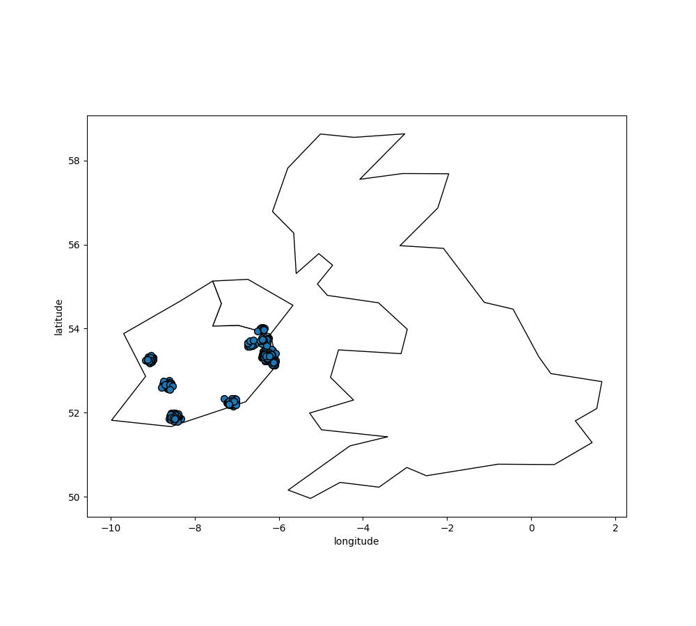
Based on the scatter plot, five seems like the optimal number of clusters. Let’s verify this hypothesis using an elbow() curve.

# Switching back to Plotly.
vp.set_option("plotting_lib", "plotly")

elbow(sm_meters, ["longitude", "latitude"], n_cluster = (3, 8))

The elbow curve seems to confirm that five is the optimal number of clusters, so let’s create a KMeans model with that in mind.

from verticapy.machine_learning.vertica import KMeans

model = KMeans(
    n_cluster = 5,
    init = [
        (-6.26980, 53.38127),
        (-9.06178, 53.25998),
        (-8.48641, 51.90216),
        (-7.12408, 52.24610),
        (-8.63985, 52.65945),
    ],
)


model.fit(
    sm_meters,
    [
        "longitude",
         "latitude",
    ],
)



=======
centers
=======
longitude|latitude
---------+--------
-9.06178 |53.25998
-8.63985 |52.65945
-8.48641 |51.90216
-7.12408 |52.24610
-6.26980 |53.38127


=======
metrics
=======
Evaluation metrics:
     Total Sum of Squares: 1209.2077
     Within-Cluster Sum of Squares: 
         Cluster 0: 0.099754154
         Cluster 1: 0.2779225
         Cluster 2: 0.53464463
         Cluster 3: 0.2657853
         Cluster 4: 17.892423
     Total Within-Cluster Sum of Squares: 19.07053
     Between-Cluster Sum of Squares: 1190.1372
     Between-Cluster SS / Total SS: 98.42%
 Number of iterations performed: 1
 Converged: True
 Call:
kmeans('"public"."_verticapy_tmp_kmeans_v_mldb_6b20cd6e97b411efa8720242ac120002_"', '"public"."_verticapy_tmp_view_v_mldb_6b9d465097b411efa8720242ac120002_"', '"longitude", "latitude"', 5
USING PARAMETERS max_iterations=300, epsilon=0.0001, initial_centers_table='"public"."_verticapy_tmp_kmeans_init_v_mldb_6bc3b5d897b411efa8720242ac120002_"', distance_method='euclidean')

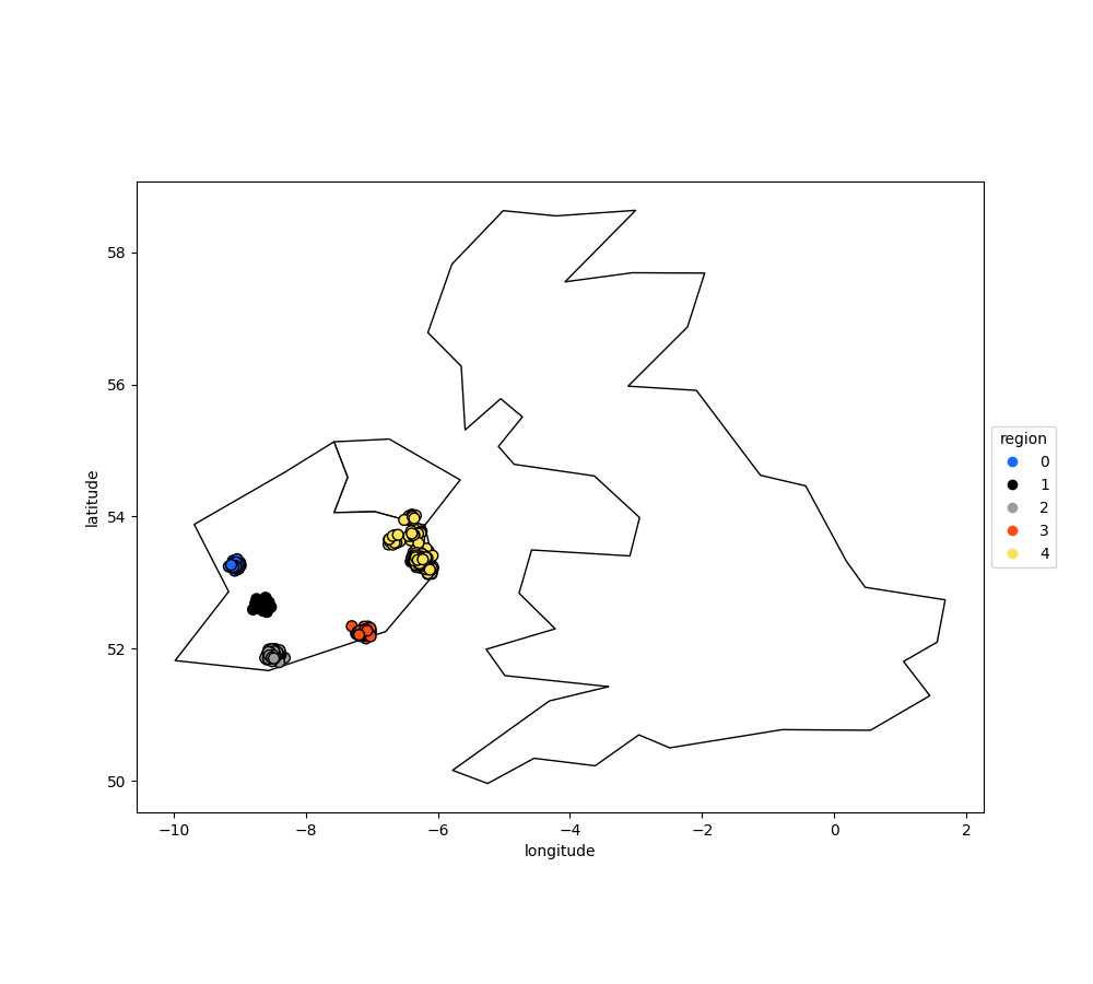
Let’s add our clusters to the vDataFrame.

sm_meters = model.predict(sm_meters, name = "region")

Let’s draw a scatter plot of the different regions.

# Geo Plots are only available in Matplotlib.
vp.set_option("plotting_lib", "matplotlib")

ax = df.plot(
    edgecolor = "black",
    color = "white",
    figsize = (10, 9),
)


sm_meters.scatter(
    ["longitude", "latitude"],
    by = "region",
    max_cardinality = 10,
    ax = ax,
)

Out[17]: <Axes: xlabel='longitude', ylabel='latitude'>

Dataset Enrichment

Let’s join sm_meters with sm_consumption_weather.

sm_consumption_weather_region = sm_consumption_weather.join(
    sm_meters,
    how = "natural",
    expr1 = ["*"],
    expr2 = [
        "residenceType",
        "region",
    ],
)
sm_consumption_weather_region.head(100)

	📅 dateUTC Timestamp(29) 100%	...	123 residenceType Integer 100%	123 region Integer 100%
1	2014-01-01 12:30:00	...	1	2
2	2014-01-01 12:30:00	...	3	4
3	2014-01-01 12:30:00	...	1	4
4	2014-01-01 12:30:00	...	3	4
5	2014-01-01 12:45:00	...	2	2
6	2014-01-01 12:45:00	...	3	4
7	2014-01-01 12:45:00	...	1	4
8	2014-01-01 12:45:00	...	1	4
9	2014-01-01 12:45:00	...	3	4
10	2014-01-01 12:45:00	...	3	0
11	2014-01-01 13:00:00	...	1	4
12	2014-01-01 13:00:00	...	3	4
13	2014-01-01 13:00:00	...	2	4
14	2014-01-01 13:00:00	...	3	2
15	2014-01-01 13:15:00	...	1	4
16	2014-01-01 13:15:00	...	1	4
17	2014-01-01 13:15:00	...	3	2
18	2014-01-01 13:15:00	...	1	0
19	2014-01-01 13:30:00	...	3	4
20	2014-01-01 13:30:00	...	1	4
21	2014-01-01 13:30:00	...	1	3
22	2014-01-01 13:30:00	...	1	4
23	2014-01-01 13:30:00	...	1	4
24	2014-01-01 13:45:00	...	3	4
25	2014-01-01 13:45:00	...	3	4
26	2014-01-01 13:45:00	...	3	2
27	2014-01-01 13:45:00	...	1	4
28	2014-01-01 14:00:00	...	1	3
29	2014-01-01 14:00:00	...	1	2
30	2014-01-01 14:00:00	...	1	4
31	2014-01-01 14:15:00	...	1	1
32	2014-01-01 14:15:00	...	1	4
33	2014-01-01 14:15:00	...	1	4
34	2014-01-01 14:15:00	...	1	2
35	2014-01-01 14:15:00	...	1	4
36	2014-01-01 14:15:00	...	2	2
37	2014-01-01 14:15:00	...	1	4
38	2014-01-01 14:30:00	...	1	4
39	2014-01-01 14:30:00	...	1	4
40	2014-01-01 14:30:00	...	1	4
41	2014-01-01 14:30:00	...	3	4
42	2014-01-01 14:45:00	...	1	4
43	2014-01-01 14:45:00	...	2	4
44	2014-01-01 14:45:00	...	1	4
45	2014-01-01 14:45:00	...	3	0
46	2014-01-01 14:45:00	...	1	4
47	2014-01-01 14:45:00	...	1	4
48	2014-01-01 15:00:00	...	1	4
49	2014-01-01 15:00:00	...	3	4
50	2014-01-01 15:00:00	...	1	3
51	2014-01-01 15:00:00	...	1	4
52	2014-01-01 15:00:00	...	1	4
53	2014-01-01 15:15:00	...	1	2
54	2014-01-01 15:15:00	...	3	4
55	2014-01-01 15:15:00	...	1	4
56	2014-01-01 15:15:00	...	1	4
57	2014-01-01 15:15:00	...	3	4
58	2014-01-01 15:15:00	...	1	2
59	2014-01-01 15:30:00	...	3	4
60	2014-01-01 15:30:00	...	1	4
61	2014-01-01 15:30:00	...	2	4
62	2014-01-01 15:30:00	...	1	3
63	2014-01-01 15:45:00	...	3	4
64	2014-01-01 15:45:00	...	1	4
65	2014-01-01 15:45:00	...	1	1
66	2014-01-01 15:45:00	...	1	2
67	2014-01-01 15:45:00	...	3	4
68	2014-01-01 16:00:00	...	3	1
69	2014-01-01 16:00:00	...	3	2
70	2014-01-01 16:00:00	...	1	3
71	2014-01-01 16:00:00	...	3	4
72	2014-01-01 16:00:00	...	1	4
73	2014-01-01 16:15:00	...	3	1
74	2014-01-01 16:15:00	...	3	4
75	2014-01-01 16:30:00	...	3	4
76	2014-01-01 16:30:00	...	1	4
77	2014-01-01 16:30:00	...	3	2
78	2014-01-01 16:30:00	...	1	4
79	2014-01-01 16:30:00	...	1	4
80	2014-01-01 16:30:00	...	2	2
81	2014-01-01 16:30:00	...	1	2
82	2014-01-01 16:45:00	...	1	4
83	2014-01-01 16:45:00	...	3	4
84	2014-01-01 17:00:00	...	1	4
85	2014-01-01 17:00:00	...	1	4
86	2014-01-01 17:00:00	...	1	4
87	2014-01-01 17:15:00	...	1	4
88	2014-01-01 17:15:00	...	3	2
89	2014-01-01 17:15:00	...	1	2
90	2014-01-01 17:15:00	...	2	2
91	2014-01-01 17:15:00	...	1	4
92	2014-01-01 17:30:00	...	2	4
93	2014-01-01 17:30:00	...	1	4
94	2014-01-01 17:30:00	...	1	4
95	2014-01-01 17:30:00	...	2	4
96	2014-01-01 17:30:00	...	1	4
97	2014-01-01 17:30:00	...	3	4
98	2014-01-01 17:30:00	...	1	2
99	2014-01-01 17:30:00	...	1	3
100	2014-01-01 17:30:00	...	2	4

Handling Missing Values

Let’s take care of our missing values.

sm_consumption_weather_region.count_percent()

	...	count	percent
"dateUTC"	...	1188432.0	100.0
"meterID"	...	1188432.0	100.0
"humidity"	...	1188432.0	100.0
"temperature"	...	1188432.0	100.0
"residenceType"	...	1188432.0	100.0
"region"	...	1188432.0	100.0
"value"	...	1188412.0	99.998

The variable value has a few missing values that we can drop.

sm_consumption_weather_region["value"].dropna()
sm_consumption_weather_region.count()

	count
"dateUTC"	1188412.0
"meterID"	1188412.0
"value"	1188412.0
"humidity"	1188412.0
"temperature"	1188412.0
"residenceType"	1188412.0
"region"	1188412.0

Interpolation & Aggregations

Since power outages seem relatively common in each area, and the value represents the electricity consumed during 30 minute intervals (in kWh), it’d be a good idea to interpolate and aggregate the data to get a monthly average in electricity consumption per region.

Let’s save our new dataset in the Vertica database.

vp.drop("sm_consumption_weather_region", method = "table")
Out[18]: True

sm_consumption_weather_region.to_db(
    "sm_consumption_weather_region",
    relation_type = "table",
)

Out[19]: 
None              dateUTC    ...    residenceType    region  
1     2014-12-30 17:00:00    ...                1         4  
2     2014-09-15 10:30:00    ...                1         4  
3     2014-09-30 18:15:00    ...                1         4  
4     2015-04-14 15:15:00    ...                1         4  
5     2015-07-05 10:30:00    ...                1         4  
6     2014-06-22 20:45:00    ...                1         4  
7     2015-09-08 16:30:00    ...                1         4  
8     2014-11-28 05:15:00    ...                1         4  
9     2014-08-11 22:00:00    ...                1         4  
10    2015-05-03 20:45:00    ...                1         4  
11    2014-08-27 16:15:00    ...                1         4  
12    2015-04-17 01:00:00    ...                1         4  
13    2014-07-05 22:45:00    ...                1         4  
14    2015-05-04 23:15:00    ...                1         4  
15    2015-04-17 09:15:00    ...                1         4  
16    2014-12-01 15:15:00    ...                1         4  
17    2014-11-13 20:00:00    ...                1         4  
18    2014-06-11 12:00:00    ...                1         4  
19    2014-04-03 15:45:00    ...                1         4  
20    2015-08-22 08:45:00    ...                1         4  
...                   ...    ...              ...       ...  
Rows: 1-20 of 1188412 | Columns: 4

sm_consumption_weather_region_clean = vp.vDataFrame("sm_consumption_weather_region")

To get an equally-sliced dataset, we can then interpolate to fill any gaps. This operation is essential for creating correct time series models.

sm_consumption_weather_region_clean = sm_consumption_weather_region_clean.interpolate(
    ts = "dateUTC",
    rule = "30 minutes",
    method = {
        "value": "linear",
        "humidity": "linear",
        "temperature": "linear",
        "residenceType": "ffill",
        "region": "ffill",
    },
    by = ["meterID"],
)
sm_consumption_weather_region_clean.head(100)

	📅 dateUTC Timestamp(29) 100%	...	123 residenceType Integer 99%	123 region Integer 99%
1	2014-01-01 05:30:00	...	[null]	[null]
2	2014-01-01 06:00:00	...	3	4
3	2014-01-01 06:30:00	...	3	4
4	2014-01-01 07:00:00	...	3	4
5	2014-01-01 07:30:00	...	3	4
6	2014-01-01 08:00:00	...	3	4
7	2014-01-01 08:30:00	...	3	4
8	2014-01-01 09:00:00	...	3	4
9	2014-01-01 09:30:00	...	3	4
10	2014-01-01 10:00:00	...	3	4
11	2014-01-01 10:30:00	...	3	4
12	2014-01-01 11:00:00	...	3	4
13	2014-01-01 11:30:00	...	3	4
14	2014-01-01 12:00:00	...	3	4
15	2014-01-01 12:30:00	...	3	4
16	2014-01-01 13:00:00	...	3	4
17	2014-01-01 13:30:00	...	3	4
18	2014-01-01 14:00:00	...	3	4
19	2014-01-01 14:30:00	...	3	4
20	2014-01-01 15:00:00	...	3	4
21	2014-01-01 15:30:00	...	3	4
22	2014-01-01 16:00:00	...	3	4
23	2014-01-01 16:30:00	...	3	4
24	2014-01-01 17:00:00	...	3	4
25	2014-01-01 17:30:00	...	3	4
26	2014-01-01 18:00:00	...	3	4
27	2014-01-01 18:30:00	...	3	4
28	2014-01-01 19:00:00	...	3	4
29	2014-01-01 19:30:00	...	3	4
30	2014-01-01 20:00:00	...	3	4
31	2014-01-01 20:30:00	...	3	4
32	2014-01-01 21:00:00	...	3	4
33	2014-01-01 21:30:00	...	3	4
34	2014-01-01 22:00:00	...	3	4
35	2014-01-01 22:30:00	...	3	4
36	2014-01-01 23:00:00	...	3	4
37	2014-01-01 23:30:00	...	3	4
38	2014-01-02 00:00:00	...	3	4
39	2014-01-02 00:30:00	...	3	4
40	2014-01-02 01:00:00	...	3	4
41	2014-01-02 01:30:00	...	3	4
42	2014-01-02 02:00:00	...	3	4
43	2014-01-02 02:30:00	...	3	4
44	2014-01-02 03:00:00	...	3	4
45	2014-01-02 03:30:00	...	3	4
46	2014-01-02 04:00:00	...	3	4
47	2014-01-02 04:30:00	...	3	4
48	2014-01-02 05:00:00	...	3	4
49	2014-01-02 05:30:00	...	3	4
50	2014-01-02 06:00:00	...	3	4
51	2014-01-02 06:30:00	...	3	4
52	2014-01-02 07:00:00	...	3	4
53	2014-01-02 07:30:00	...	3	4
54	2014-01-02 08:00:00	...	3	4
55	2014-01-02 08:30:00	...	3	4
56	2014-01-02 09:00:00	...	3	4
57	2014-01-02 09:30:00	...	3	4
58	2014-01-02 10:00:00	...	3	4
59	2014-01-02 10:30:00	...	3	4
60	2014-01-02 11:00:00	...	3	4
61	2014-01-02 11:30:00	...	3	4
62	2014-01-02 12:00:00	...	3	4
63	2014-01-02 12:30:00	...	3	4
64	2014-01-02 13:00:00	...	3	4
65	2014-01-02 13:30:00	...	3	4
66	2014-01-02 14:00:00	...	3	4
67	2014-01-02 14:30:00	...	3	4
68	2014-01-02 15:00:00	...	3	4
69	2014-01-02 15:30:00	...	3	4
70	2014-01-02 16:00:00	...	3	4
71	2014-01-02 16:30:00	...	3	4
72	2014-01-02 17:00:00	...	3	4
73	2014-01-02 17:30:00	...	3	4
74	2014-01-02 18:00:00	...	3	4
75	2014-01-02 18:30:00	...	3	4
76	2014-01-02 19:00:00	...	3	4
77	2014-01-02 19:30:00	...	3	4
78	2014-01-02 20:00:00	...	3	4
79	2014-01-02 20:30:00	...	3	4
80	2014-01-02 21:00:00	...	3	4
81	2014-01-02 21:30:00	...	3	4
82	2014-01-02 22:00:00	...	3	4
83	2014-01-02 22:30:00	...	3	4
84	2014-01-02 23:00:00	...	3	4
85	2014-01-02 23:30:00	...	3	4
86	2014-01-03 00:00:00	...	3	4
87	2014-01-03 00:30:00	...	3	4
88	2014-01-03 01:00:00	...	3	4
89	2014-01-03 01:30:00	...	3	4
90	2014-01-03 02:00:00	...	3	4
91	2014-01-03 02:30:00	...	3	4
92	2014-01-03 03:00:00	...	3	4
93	2014-01-03 03:30:00	...	3	4
94	2014-01-03 04:00:00	...	3	4
95	2014-01-03 04:30:00	...	3	4
96	2014-01-03 05:00:00	...	3	4
97	2014-01-03 05:30:00	...	3	4
98	2014-01-03 06:00:00	...	3	4
99	2014-01-03 06:30:00	...	3	4
100	2014-01-03 07:00:00	...	3	4

Let’s aggregate the data to figure out the monthly energy consumption for each smart meter. We can then save the result in the Vertica database.

import verticapy.sql.functions as fun

sm_consumption_weather_region_clean["month"] = "MONTH(dateUTC)"
sm_consumption_weather_region_clean["date_month"] = "DATE_TRUNC('MONTH', dateUTC::date)"
sm_consumption_month = sm_consumption_weather_region_clean.groupby(
    columns = [
        "meterID",
        "region",
        "residenceType",
        "month",
        "date_month",
    ],
    expr = [
        fun.sum(sm_consumption_weather_region["value"])._as("value"),
        fun.avg(sm_consumption_weather_region["temperature"])._as("avg_temperature"),
        fun.avg(sm_consumption_weather_region["humidity"])._as("avg_humidity"),
    ],
).filter(
    "date_month < '2015-09-01'",
)
vp.drop("sm_consumption_month", method = "table")
sm_consumption_month.to_db(
    "sm_consumption_month",
    relation_type = "table",
    inplace = True,
)

	123 meterID Int 100%	...	123 region Int 97%	123 avg_humidity Float 97%
1	2	...	[null]	[null]
2	2	...	4	84.9491344603949
3	2	...	4	94.0992998737685
4	2	...	4	86.0871432645725
5	2	...	4	90.4227418530055
6	2	...	4	80.8285802271696
7	2	...	4	82.2095048876506
8	2	...	4	85.081830737512
9	2	...	4	77.0781891119151
10	2	...	4	84.3597425444918
11	2	...	4	78.7060994156184
12	2	...	4	82.169875343245
13	2	...	4	80.3458444814076
14	2	...	4	83.3348880025485
15	2	...	4	79.4181890210453
16	2	...	4	84.0634813017688
17	2	...	4	81.8807510916972
18	2	...	4	84.3442042309829
19	2	...	4	86.9737490248736
20	2	...	4	87.2311202524699

Understanding the Data & Detecting Outliers

Looking at three different smart meters, we can see a clear decrease in energy consumption during the summer followed by a sharp increase in the winter.

# Switching back to Plotly.
vp.set_option("plotting_lib", "plotly")

sm_consumption_month[sm_consumption_month["meterID"] == 10]["value"].plot(ts = "date_month")

sm_consumption_month[sm_consumption_month["meterID"] == 12]["value"].plot(ts = "date_month")

sm_consumption_month[sm_consumption_month["meterID"] == 14]["value"].plot(ts = "date_month")

This behavior seems to be seasonal, but we don’t have enough data to prove this.

Let’s find outliers in the distribution by computing the ZSCORE` per meterID.

std = fun.std(sm_consumption_month["value"])._over(by = [sm_consumption_month["meterID"]])
avg = fun.avg(sm_consumption_month["value"])._over(by = [sm_consumption_month["meterID"]])
sm_consumption_month["value_zscore"] = (sm_consumption_month["value"] - avg) / std
sm_consumption_month.search("value_zscore > 4")

	123 meterID Integer 100%	...	123 avg_humidity Float(22) 100%	123 value_zscore Float(22) 100%
1	399	...	88.7730360914782	4.07298404322647
2	364	...	89.9652523028262	4.00855200430863
3	809	...	86.4715802984117	4.0151606376986
4	951	...	73.6313461768108	4.01829822269677

Four smart meters are outliers in energy consumption. We’ll need to investigate to get more information.

sm_consumption_month[sm_consumption_month["meterID"] == 364]["value"].plot(ts = "date_month")

sm_consumption_month[sm_consumption_month["meterID"] == 399]["value"].plot(ts = "date_month")

sm_consumption_month[sm_consumption_month["meterID"] == 809]["value"].plot(ts = "date_month")

sm_consumption_month[sm_consumption_month["meterID"] == 951]["value"].plot(ts = "date_month")

Data Encoding & Bivariate Analysis

Since most of our data is categorical, let’s encode them with One-hot encoding. We can then examine the correlations between the various categories.

sm_consumption_month = sm_consumption_month.one_hot_encode(
    ["region", "residenceType", "month"],
    drop_first = False,
    max_cardinality = 20,
)
sm_consumption_month.head(100)

	123 meterID Int 100%	...	123 month_11 Bool 100%	123 month_12 Bool 100%
1	2	...	0	0
2	2	...	0	0
3	2	...	0	0
4	2	...	0	0
5	2	...	0	0
6	2	...	0	0
7	2	...	0	0
8	2	...	0	0
9	2	...	0	0
10	2	...	0	0
11	2	...	0	0
12	2	...	0	0
13	2	...	0	0
14	2	...	0	0
15	2	...	0	0
16	2	...	0	0
17	2	...	0	0
18	2	...	0	0
19	2	...	0	0
20	2	...	1	0
21	2	...	0	1
22	3	...	0	0
23	3	...	0	0
24	3	...	0	0
25	3	...	0	0
26	3	...	0	0
27	3	...	0	0
28	3	...	0	0
29	3	...	0	0
30	3	...	0	0
31	3	...	0	0
32	3	...	0	0
33	3	...	0	0
34	3	...	0	0
35	3	...	0	0
36	3	...	0	0
37	3	...	0	0
38	3	...	0	0
39	3	...	0	0
40	3	...	1	0
41	3	...	0	1
42	16	...	0	0
43	16	...	0	0
44	16	...	0	0
45	16	...	0	0
46	16	...	0	0
47	16	...	0	0
48	16	...	0	0
49	16	...	0	0
50	16	...	0	0
51	16	...	0	0
52	16	...	0	0
53	16	...	0	0
54	16	...	0	0
55	16	...	0	0
56	16	...	0	0
57	16	...	0	0
58	16	...	0	0
59	16	...	0	0
60	16	...	0	0
61	16	...	1	0
62	16	...	0	1
63	25	...	0	0
64	25	...	0	0
65	25	...	0	0
66	25	...	0	0
67	25	...	0	0
68	25	...	0	0
69	25	...	0	0
70	25	...	0	0
71	25	...	0	0
72	25	...	0	0
73	25	...	0	0
74	25	...	0	0
75	25	...	0	0
76	25	...	0	0
77	25	...	0	0
78	25	...	0	0
79	25	...	0	0
80	25	...	0	0
81	25	...	1	0
82	25	...	0	1
83	30	...	0	0
84	30	...	0	0
85	30	...	0	0
86	30	...	0	0
87	30	...	0	0
88	30	...	0	0
89	30	...	0	0
90	30	...	0	0
91	30	...	0	0
92	30	...	0	0
93	30	...	0	0
94	30	...	0	0
95	30	...	0	0
96	30	...	0	0
97	30	...	0	0
98	30	...	0	0
99	30	...	0	0
100	30	...	0	0

Let’s compute the Pearson correlation matrix.

sm_consumption_month.corr()

There’s a clear correlation between the month and energy consumption, but this isn’t causal. Instead, we can think of the weather as having the direct influence on energy consumption. To accomodate for this view, we’ll use the temperature as a predictor (rather than the month).

sm_consumption_month.corr(focus = "value")

Global Behavior

Let’s look at this globally.

sm_consumption_final = sm_consumption_month.groupby(
    ["date_month"],
    [
        fun.avg(sm_consumption_month["avg_temperature"])._as("avg_temperature"),
        fun.avg(sm_consumption_month["avg_humidity"])._as("avg_humidity"),
        fun.avg(sm_consumption_month["value"])._as("avg_value"),
    ],
)
sm_consumption_final.plot(ts = "date_month", columns = ["avg_value"])

We expect to see a fall in energy consumption during summer and then an increase during the winter. A simple prediction could use the average value a year before.

sm_consumption_final["prediction"] = fun.case_when(
    sm_consumption_final["date_month"] < '2015-01-01', sm_consumption_final["avg_value"],
    fun.lag(sm_consumption_final["avg_value"], 12)._over(order_by = ["date_month"]),
)
sm_consumption_final.plot(ts = "date_month", columns = ["prediction", "avg_value"])

sm_consumption_final.score("avg_value", "prediction", "r2")
Out[21]: 0.987990336935642

As expected, our model’s score is excellent.

Let’s use machine learning to understand the influence of the weather and the humidity on energy consumption.

Machine Learning

Let’s create our model.

from verticapy.machine_learning.vertica import LinearRegression

predictors = [
    "avg_temperature",
    "avg_humidity",
]


model = LinearRegression(solver = "BFGS")

model.fit(
    sm_consumption_final,
    predictors,
    "avg_value",
)



=======
details
=======
   predictor   |coefficient| std_err |t_value |p_value 
---------------+-----------+---------+--------+--------
   Intercept   | 150.86469 |228.92349| 0.65902| 0.51871
avg_temperature| -4.09012  | 1.13606 |-3.60026| 0.00221
 avg_humidity  |  6.41306  | 2.22558 | 2.88152| 0.01036


==============
regularization
==============
type| lambda 
----+--------
none| 1.00000


===========
call_string
===========
linear_reg('"public"."_verticapy_tmp_linearregression_v_mldb_91ad5ec097b411efa8720242ac120002_"', '"public"."_verticapy_tmp_view_v_mldb_92201ee297b411efa8720242ac120002_"', '"avg_value"', '"avg_temperature", "avg_humidity"'
USING PARAMETERS optimizer='bfgs', epsilon=1e-06, max_iterations=100, regularization='none', lambda=1, alpha=0.5, fit_intercept=true)

===============
Additional Info
===============
       Name       |Value
------------------+-----
 iteration_count  |  4  
rejected_row_count|  0  
accepted_row_count| 20  

model.report("details")

	value
Dep. Variable	"avg_value"
Model	LinearRegression
No. Observations	20.0
No. Predictors	2
R-squared	0.799113694213527
Adj. R-squared	0.7754800111798242
F-statistic	33.81249096905822
Prob (F-statistic)	3.837253952408338e-07
Kurtosis	-0.0457129692472424
Skewness	0.893296166786592
Jarque-Bera (JB)	3.65140760780652

The model seems to be good with an adjusted R2 of 77.5%, and the F-Statistic indicates that at least one of the two predictors is useful. Let’s look at the residual plot.

sm_consumption_final = model.predict(
    sm_consumption_final,
    name = "value_prediction",
)
sm_consumption_final["residual"] = sm_consumption_final["avg_value"] - sm_consumption_final["value_prediction"]
sm_consumption_final.scatter(["avg_value", "residual"])

Looking at the residual plot, we can see that the error variance varies by quite a bit. A possible suspect might be heteroscedasticity. Let’s verify our hypothesis using a Breusch-Pagan test.

from verticapy.machine_learning.model_selection.statistical_tests import het_breuschpagan

het_breuschpagan(sm_consumption_final, "residual", predictors)
Out[27]: 
(6.066154825831241,
 0.04816717950866987,
 3.700508752254135,
 0.04632851414387972)

The p-value is 4.81% and sits around the 5% threshold, so we can’t really draw any conclusions.

Let’s look at the entire regression report.

model.report()

	value
explained_variance	0.799113694213527
max_error	64.4503700445752
median_absolute_error	13.1054316247273
mean_absolute_error	20.9034976459432
mean_squared_error	734.33259460088
root_mean_squared_error	27.0985718184719
r2	0.799113694213527
r2_adj	0.775480011179824
aic	140.604241042862
bic	140.966437863524

Our model is very good; its median absolute error is around 13kWh. With this model, we can make predictions about the energy consumption of households per region. If the usage exceeds what the model predicts, we can raise an alert and respond, for example, by regulating the electricity distributed to the region.

Conclusion

We’ve solved our problem in a Pandas-like way, all without ever loading data into memory!