Pivot Table
General
Let’s begin by importing verticapy.
import verticapy as vp
Let’s also import numpy to create a random dataset.
import numpy as np
Let’s generate a dataset using the following data.
N = 100 # Number of records
data = vp.vDataFrame({
"category1": [np.random.choice(['A','B','C']) for _ in range(N)],
"category2": [np.random.choice(['D','E']) for _ in range(N)],
"score1": np.random.normal(10, 2, N),
"score2": np.random.normal(5, 1.5, N),
})
In the context of data visualization, we have the flexibility to harness multiple plotting libraries to craft a wide range of graphical representations. VerticaPy, as a versatile tool, provides support for several graphic libraries, such as Matplotlib, Highcharts, and Plotly. Each of these libraries offers unique features and capabilities, allowing us to choose the most suitable one for our specific data visualization needs.

Note
To select the desired plotting library, we simply need to use the set_option() function. VerticaPy offers the flexibility to smoothly transition between different plotting libraries. In instances where a particular graphic is not supported by the chosen library or is not supported within the VerticaPy framework, the tool will automatically generate a warning and then switch to an alternative library where the graphic can be created.
Please click on the tabs to view the various graphics generated by the different plotting libraries.
We can switch to using the plotly module.
vp.set_option("plotting_lib", "plotly")
VerticaPy has the capability to calculate comprehensive pivot tables and can also automatically discretize and group numerical features, simplifying the data analysis process.
data.pivot_table(columns = ["category1", "category2"])
We load the VerticaPy chart extension.
%load_ext verticapy.chart
We write the SQL query using Jupyter magic cells.
%%chart -k spider
SELECT category1, category2, COUNT(*) FROM :data GROUP BY 1, 2;
We can switch to using the highcharts module.
vp.set_option("plotting_lib", "highcharts")
VerticaPy has the capability to calculate comprehensive pivot tables and can also automatically discretize and group numerical features, simplifying the data analysis process.
data.pivot_table(columns = ["category1", "category2"])
We load the VerticaPy chart extension.
%load_ext verticapy.chart
We write the SQL query using Jupyter magic cells.
%%chart -k spider
SELECT category1, category2, COUNT(*) FROM :data GROUP BY 1, 2;
We can switch to using the matplotlib module.
vp.set_option("plotting_lib", "matplotlib")
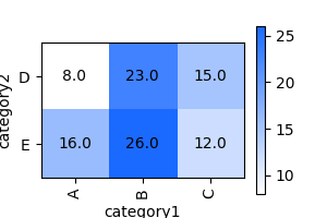
VerticaPy has the capability to calculate comprehensive pivot tables and can also automatically discretize and group numerical features, simplifying the data analysis process.
data.pivot_table(columns = ["category1", "category2"])
Out[3]: <Axes: xlabel='category1', ylabel='category2'>
We load the VerticaPy chart extension.
%load_ext verticapy.chart
We write the SQL query using Jupyter magic cells.
%%chart -k spider
SELECT category1, category2, COUNT(*) FROM :data GROUP BY 1, 2;
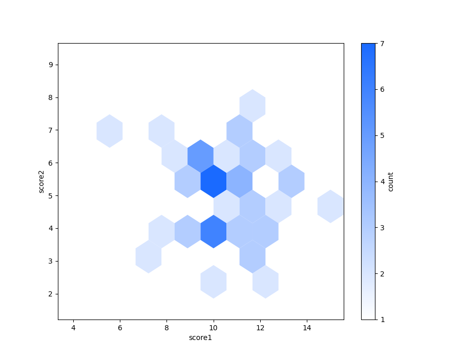
data.hexbin(columns = ["score1", "score2"])
Out[4]: <Axes: xlabel='score1', ylabel='score2'>
Custom Aggregations
Within the VerticaPy framework, you have the flexibility to apply a wide array of aggregation techniques according to your specific analytical needs. This extends to the option of utilizing SQL statements, allowing you to craft custom aggregations that precisely match your data summarization requirements. VerticaPy empowers you with the versatility to aggregate data in the manner that best serves your analytical objectives.
Note
In SQL, aggregations can be computed directly within the input SQL statement, but in Python, the process is a bit different.
General Options
data.pivot_table(columns = ["category1", "category2"], method = "count", of = "score1")
Hint
VerticaPy simplifies the usage of aggregations, such as percentiles. You only need to specify the percentile number without a decimal point to compute it. For instance, 50% for the median, 75% for the third quartile, and 99% for the last percentile.
Direct SQL statement
Note
You are free to utilize any SQL statement as long as it is compatible with the supported features of VerticaPy.
data.pivot_table(columns = ["category1", "category2"], method = "COUNT(score1) AS count_score")
General Options
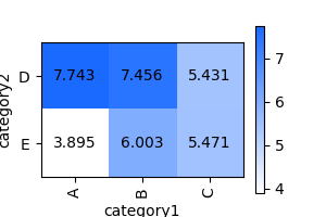
data.pivot_table(columns = ["category1", "category2"], method = "min", of = "score1")
Hint
VerticaPy simplifies the usage of aggregations, such as percentiles. You only need to specify the percentile number without a decimal point to compute it. For instance, 50% for the median, 75% for the third quartile, and 99% for the last percentile.
Direct SQL statement
Note
You are free to utilize any SQL statement as long as it is compatible with the supported features of VerticaPy.
data.pivot_table(columns = ["category1", "category2"], method = "MIN(score1) AS min_score")
General Options
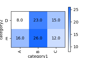
data.pivot_table(columns = ["category1", "category2"], method = "min", of = "score1")
Out[5]: <Axes: xlabel='category1', ylabel='category2'>
Hint
VerticaPy simplifies the usage of aggregations, such as percentiles. You only need to specify the percentile number without a decimal point to compute it. For instance, 50% for the median, 75% for the third quartile, and 99% for the last percentile.
Direct SQL statement
Note
You are free to utilize any SQL statement as long as it is compatible with the supported features of VerticaPy.
data.pivot_table(columns = ["category1", "category2"], method = "MIN(score1) AS min_score")
Out[6]: <Axes: xlabel='category1', ylabel='category2'>
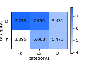
Chart Customization
VerticaPy empowers users with a high degree of flexibility when it comes to tailoring the visual aspects of their plots. This customization extends to essential elements such as color schemes, text labels, and plot sizes, as well as a wide range of other attributes that can be fine-tuned to align with specific design preferences and analytical requirements. Whether you want to make your visualizations more visually appealing or need to convey specific insights with precision, VerticaPy’s customization options enable you to craft graphics that suit your exact needs.
Hint
For SQL users who use Jupyter Magic cells, chart customization must be done in Python. They can then export the graphic using the last magic cell result.
chart = _
Now, the chart variable includes the graphic. Depending on the library you are using, you will obtain a different object.
Important
Different customization parameters are available for Plotly, Highcharts, and Matplotlib. For a comprehensive list of customization features, please consult the documentation of the respective libraries: plotly, matplotlib and highcharts.
Colors
Custom CMAP
data.pivot_table(columns = ["category1", "category2"], color_continuous_scale = [[0, "white"], [1, "red"]])
Custom CMAP
fig = data.pivot_table(columns = ["category1", "category2"])
fig.set_options(
"colorAxis",
{
"stops": [
[0, "white"],
[0.45, "yellow"],
[0.55, "pink"],
[1, "red"],
],
"min": -1,
"max": 1,
},
)
fig
Custom CMAP
data.pivot_table(columns = ["category1", "category2"], cmap = "Reds")
Out[7]: <Axes: xlabel='category1', ylabel='category2'>

Size
Custom Width and Height
data.pivot_table(columns = ["category1", "category2"], width = 300, height = 300)
Custom Width and Height
data.pivot_table(columns = ["category1", "category2"], width = 500, height = 200)
Custom Width and Height
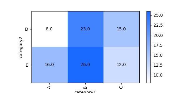
data.pivot_table(columns = ["category1", "category2"], width = 6, height = 3)
Out[8]: <Axes: xlabel='category1', ylabel='category2'>
Text
Custom Title
data.pivot_table(columns = ["category1", "category2"]).update_layout(title_text = "Custom Title")
Custom Axis Titles
data.pivot_table(columns = ["category1", "category2"], yaxis_title = "Custom Y-Axis Title")
Custom Title Text
data.pivot_table(columns = ["category1", "category2"], title = {"text": "Custom Title"})
Custom Axis Titles
data.pivot_table(columns = ["category1", "category2"], xAxis = {"title": {"text": "Custom X-Axis Title"}})
Custom Title Text
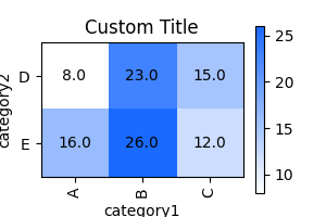
data.pivot_table(columns = ["category1", "category2"]).set_title("Custom Title")
Out[9]: Text(0.5, 1.0, 'Custom Title')
Custom Axis Titles
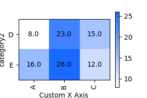
data.pivot_table(columns = ["category1", "category2"]).set_xlabel("Custom X Axis")
Out[10]: Text(0.5, 0, 'Custom X Axis')