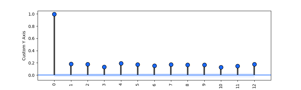
Auto-Correlation Plot
General
Let’s begin by importing verticapy.
import verticapy as vp
Let’s import the amazon dataset from verticapy.
from verticapy.datasets import load_amazon
data = load_amazon()
In the context of data visualization, we have the flexibility to harness multiple plotting libraries to craft a wide range of graphical representations. VerticaPy, as a versatile tool, provides support for several graphic libraries, such as Matplotlib, Highcharts, and Plotly. Each of these libraries offers unique features and capabilities, allowing us to choose the most suitable one for our specific data visualization needs.

Note
To select the desired plotting library, we simply need to use the set_option() function. VerticaPy offers the flexibility to smoothly transition between different plotting libraries. In instances where a particular graphic is not supported by the chosen library or is not supported within the VerticaPy framework, the tool will automatically generate a warning and then switch to an alternative library where the graphic can be created.
Please click on the tabs to view the various graphics generated by the different plotting libraries.
We can switch to using the plotly module.
vp.set_option("plotting_lib", "plotly")
Hint
In VerticaPy, you have access to a variety of correlation techniques, including Pearson for linear relationships, Spearman for monotonic relationships, Cramer’s V for categorical data, and more. It’s important to note that each of these techniques involves SQL generation and may vary in computational cost. You can choose the most suitable technique based on your analysis requirements, considering the potential computational overhead.
data.acf(column = "number", ts = "date", by= "state",
method = "pearson", p=48,
)
data.acf(column = "number", ts = "date", by= "state", method = "pearson", kind = "heatmap")
We can switch to using the highcharts module.
vp.set_option("plotting_lib", "highcharts")
Hint
In VerticaPy, you have access to a variety of correlation techniques, including Pearson for linear relationships, Spearman for monotonic relationships, Cramer’s V for categorical data, and more. It’s important to note that each of these techniques involves SQL generation and may vary in computational cost. You can choose the most suitable technique based on your analysis requirements, considering the potential computational overhead.
data.acf(column = "number", ts = "date", by= "state",
method = "pearson", p=48,
)
data.acf(column = "number", ts = "date", by= "state", method = "pearson", kind = "heatmap")
We can switch to using the matplotlib module.
vp.set_option("plotting_lib", "matplotlib")
Hint
In VerticaPy, you have access to a variety of correlation techniques, including Pearson for linear relationships, Spearman for monotonic relationships, Cramer’s V for categorical data, and more. It’s important to note that each of these techniques involves SQL generation and may vary in computational cost. You can choose the most suitable technique based on your analysis requirements, considering the potential computational overhead.
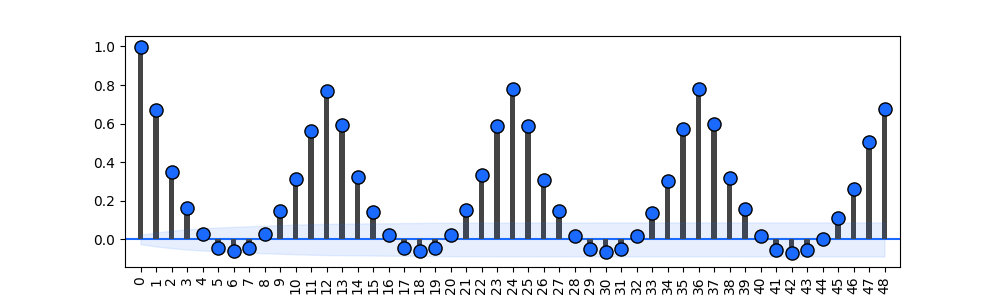
data.acf(column = "number", ts = "date", by= "state",
method = "pearson", p=48,
)
Out[2]: <Axes: xlabel='lag'>
data.acf(column = "number", ts = "date", by= "state", method = "pearson", kind = "heatmap")
Out[3]: <Axes: >

Chart Customization
VerticaPy empowers users with a high degree of flexibility when it comes to tailoring the visual aspects of their plots. This customization extends to essential elements such as color schemes, text labels, and plot sizes, as well as a wide range of other attributes that can be fine-tuned to align with specific design preferences and analytical requirements. Whether you want to make your visualizations more visually appealing or need to convey specific insights with precision, VerticaPy’s customization options enable you to craft graphics that suit your exact needs.
Important
Different customization parameters are available for Plotly, Highcharts, and Matplotlib. For a comprehensive list of customization features, please consult the documentation of the respective libraries: plotly, matplotlib and highcharts.
Colors
Custom Colors
data.acf(column = "number", ts = "date", method = "pearson", colors = "red")
Custom Colors
data.acf(column = "number", ts = "date", method = "pearson", colors = "red")
Custom Colors
data.acf(column = "number", ts = "date", method = "pearson", colors = "red")
Out[4]: <Axes: xlabel='lag'>

Size
Custom Width and Height
data.acf(column = "number", ts = "date", method = "pearson", width = 300, height = 300)
Custom Width and Height
data.acf(column = "number", ts = "date", method = "pearson", width = 500, height = 200)
Custom Width and Height
data.acf(column = "number", ts = "date", method = "pearson", width = 6, height = 3)
Out[5]: <Axes: xlabel='lag'>

Text
Custom Title
data.acf(column = "number", ts = "date", method = "pearson").update_layout(title_text = "Custom Title")
Custom Axis Titles
data.acf(column = "number", ts = "date", method = "pearson", yaxis_title = "Custom Y-Axis Title")
Custom Title Text
data.acf(column = "number", ts = "date", method = "pearson", title = {"text": "Custom Title"})
Custom Axis Titles
data.acf(column = "number", ts = "date", method = "pearson", xAxis = {"title": {"text": "Custom X-Axis Title"}})
Custom Title Text
data.acf(column = "number", ts = "date", method = "pearson").set_title("Custom Title")
Out[6]: Text(0.5, 1.0, 'Custom Title')
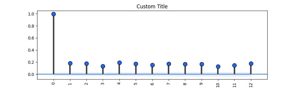
Custom Axis Titles
data.acf(column = "number", ts = "date", method = "pearson").set_ylabel("Custom Y Axis")
Out[7]: Text(0, 0.5, 'Custom Y Axis')