End-To-End Data Transformation Guide: Using the dbt-vertica Adapter for Analytics
This video explains the integration of dbt and Vertica using the open-source dbt-vertica-adapter. Check out the video to understand how you can quickly transform your raw data directly in Vertica and take advantage of the new features in the adapter.
dbt or Data Build Tool, is a data transformation tool that streamlines the process of transforming raw data into curated data sets that are clean, easy to query, and ready for analysis. In dbt, data transformations and business logic are expressed using SQL statements and Jinja language. Jinja turns dbt into a programing environment for SQL.
You can use dbt and OpenText™ Vertica™ to build a robust and efficient data transformation pipeline. dbt code is processed in-database leveraging Vertica’s high performance. In addition, dbt provides software development best practices such as, version control, built-in testing framework, documentation, and code reusability that allows SQL developers to work like Software Engineers.
The dbt adapter for Vertica enables the connection to Vertica from dbt. dbt-vertica is an open-source project available in Vertica’s GitHub repository. It is written in Python and yml, and uses the vertica-python driver.
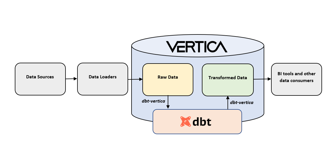
Vertica + dbt Data Stack
This is a diagram of dbt and Vertica data stack. dbt transforms data that is already loaded into Vertica and uses the dbt-vertica adapter to connect to your database. Unlike traditional data transformation tools, dbt data transformations are executed directly in your database. No data is transferred out of Vertica. The transformed data can then be used by BI tools and other technologies for further analysis.
Solution Overview
This document provides an example of a data transformation pipeline using VMart and includes the steps to configure the environment and connect to Vertica using the dbt-vertica adapter.
The solution presented in this document is categorized in the following sections:
You can expand and collapse topics for more details as you go along reading the guide.
Scope
Familiarity with dbt-core, Vertica, SQL, Jinja, and VS Code is required and assumed.
This document does not cover
-
Installation of Vertica and the VMart database.
-
Data loading: The process to load the raw data into Vertica.
-
Data visualization: The steps to visualize the transformed data.
-
dbt cloud.
Environment
This is the environment we used to execute the examples in this document:
Important dbt-core and vertica-python are automatically installed when you install the dbt-vertica adapter.
-
Vertica Analytical Database 23.3.0 installed on a 3-node Linux VM cluster.
-
VMart example database
-
Visual Studio Code (vscode) version 1.76.2
-
git version 2.40.0
-
python version 3.11.2
-
dbt-vertica adapter version 1.5.0
-
vertica-python driver version 1.3.1
-
dbt-core version 1.5.0
-
In our testing, we used DBVisualizer version 13.0.4 to examine the data in tables or views in a user-friendly manner.
Vertica environment:
dbt environment on Windows:
A database SQL client that can connect to the database:
Configuring the Environment to Use dbt with Vertica
This section explains how to install the dbt-vertica adapter and initialize a dbt project. The configuration is based on a Windows environment.
Ensure you have installed the following before you begin:
-
python
-
git
Note git is recommended to incorporate source control in your dbt project. This is a best practices. Make sure to add an entry of the location of git.exe to the user’s path environment variable.
-
Visual Studio Code (VS Code)
-
VS Code Python extension
Follow these steps to install the adapter on Windows:
-
Open VS Code.
-
In the Terminal menu at the top of the screen, click New Terminal.
-
The command line interface CLI opens up.
-
Create and activate a Python Virtual Environment.
Note We recommend you to install the adapter and create your dbt project in this isolated environment.
-
Move to the folder where you want to create your virtual environment, and create and activate your environment:

-
Run a pip install dbt-vertica to install the adapter:
Note This action installs dbt-core and vertica-python, you do not need to install them separately.
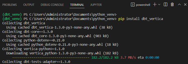
The log should end with the list of packages that got installed like this:

Follow these steps to initialize the dbt project that will host your transformation models:
-
Create a folder to host the dbt project and run the dbt init command to create the project in this location. Enter the information requested in the CLI:
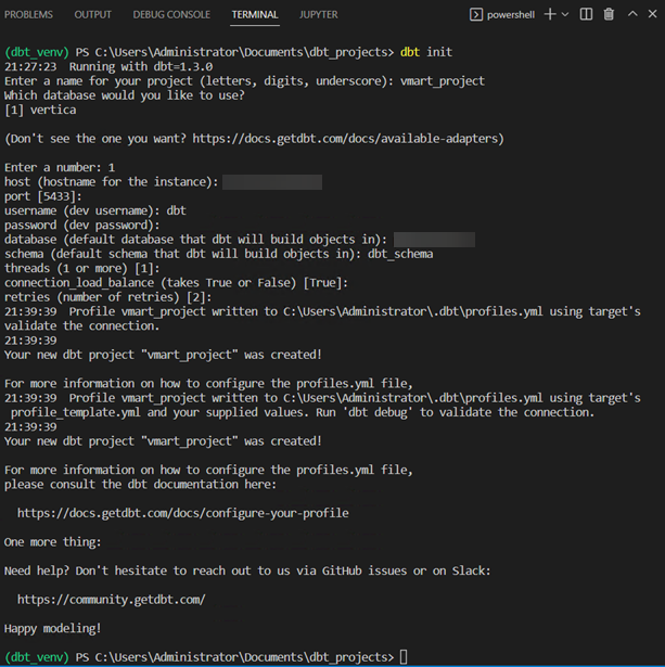
Note This action creates a skeleton project with all the necessary empty folders. It also creates the profile file you can edit to connect to Vertica. The dbt project file dbt_project.yml contains the project configuration.
Configuring a dbt Profile to Connect to Vertica
This section explains how you can configure the connection to Vertica also known as the dbt profile. The dbt profiles file is generated automatically when you initialize a project as described in the previous section. The dbt profiles file is in the following directory: C:\Users\<my_user>\.dbt\profiles.yml.
Below is an example of the profiles file profiles.yml. You can edit the profiles file and add multiple connections identified by a unique name. The connection you used in your project is specified in the project configuration file dbt_project.yml.
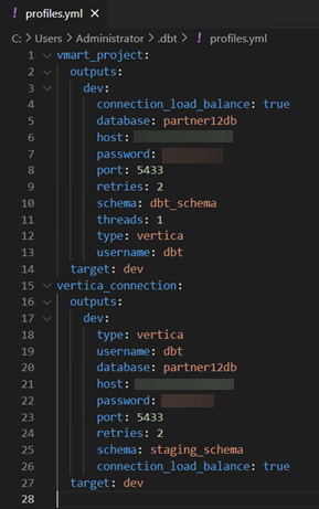
Execute the dbt debug command to test your connection to Vertica. This command should be run with the Python virtual environment active and inside the folder of your dbt project.
Note dbt debug checks that python and all .yml files have been configured correctly and that dbt is able to reach Vertica using the connection information provided in the profiles.yml file.
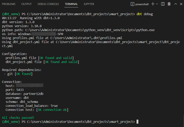
When all tests have passed, you are ready to start building your dbt models.
Example of a Data Transformation Pipeline Using VMart
The following solution consists of a data transformation pipeline with the purpose of business analytics and reporting. We want to calculate the on-time delivery rate, quantity accuracy rate, and the perfect order rate by vendor. We will call this final model vendor_performance. We will show how the vendor_performance model is created throughout a series of transformation steps that begin with the raw data.
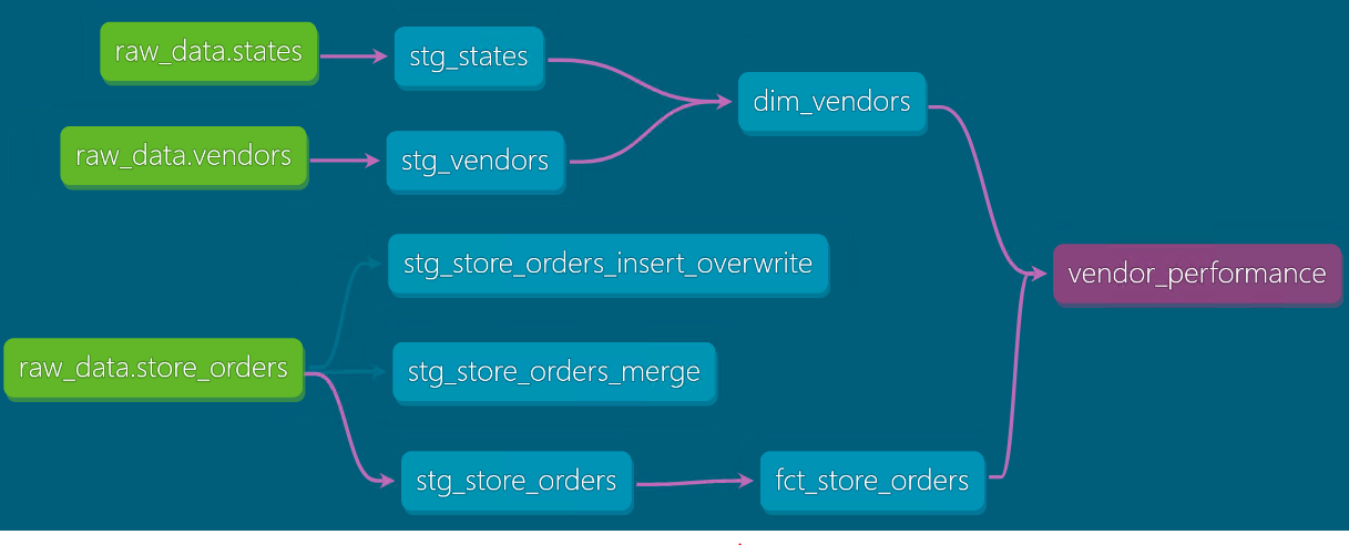
This is the Lineage graph of the solution. It represents the flow of data from source to final model:
-
The green nodes are the sources/raw data that we use in this project.
-
The second level of nodes are the staging models that reference the sources and slightly transform the raw data.
-
Third level of nodes are the models that reference the staging models and apply business logic to transform them. In this case a dimension and a fact table. Users might query these models using a BI tool.
-
Last node is the final model that uses both the fact table and the dimension table and calculates Vendor KPIs for reporting.
The project is organized using the following folder structure:
-
staging: Contains the models that reference the raw data tables and slightly transform them.
-
marts > vmart: Contains the models that reference the staging models and apply business logic to further transform them.
-
reports: Contains the final models that end-users may query for analysis.
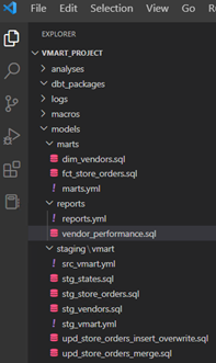
The source is the raw data that we process in the project. The source file for this project is src_vmart.yml in the models > staging > vmart directory. This file documents and specifies the tests for the following raw tables: raw_schema.states, raw_schema.vendors, and raw_schema.store_orders:

Note You can use Vertica’s built-in functionality or various complementary technologies to bring source data into your database. Source data along with ddl files reside in the demo_dbt_vmart/sampledata directory. The raw data used in this project has been already loaded into Vertica.
models > staging > vmart > src_vmart.yml
version: 2

sources:
  - name: raw_data
    description: This is the raw data to transform.
    database: partner12db
    schema: raw_schema
    tables:
      - name: states
        description: This is the raw states data.
        columns:
          - name: statecode
            description: The primary key for the raw states data.
            tests:
              - unique
              - not_null

      - name: vendors
        description: This is the raw vendors data.
        columns:
          - name: vendorid
            description: The primary key for the raw vendors data.
            tests:
              - unique
              - not_null

      - name: store_orders
        description: This is the raw store_orders data.
        columns:
          - name: ordernumber
            description: The primary key for the raw store_orders data.
            tests:
              - unique
              - not_null
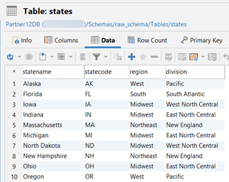
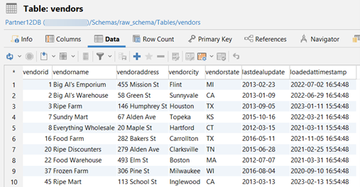
This is what the data looks like for each raw table. The images display only the first 10 rows of data:
raw_schema.states:
raw_ schema.vendors:
raw_ schema.store_orders:

A dbt model is a select statement that we write in a SQL file with the purpose of transforming data.
The following staging models standardize the column names in the raw tables and are in the models > staging > vmart directory.
Note These models are built as views.
models > staging > vmart > stg_vendors.sql
This model creates the dbt_schema.stg_vendors view. It references the raw data table vendors.
with source as (
    select * from {{ source('raw_data', 'vendors') }}
),

staged as (
    select
        vendorid as vendor_key,
        vendorname as vendor_name,
        vendoraddress as vendor_address,
        vendorcity as vendor_city,
        vendorstate as vendor_state,
        lastdealupdate as last_deal_update,
        loadedattimestamp as loaded_at_timestamp
    from source
)

select * from staged
models > staging > vmart > stg_states.sql
This model creates the dbt_schema.stg_states view. It references the raw data table states.
with source as (
    select * from {{ source('raw_data', 'states') }}
),

staged as (
    select
        statename as state_name,
        statecode as state_code,
        region,
        division
    from source
)

select * from staged
models > staging > vmart > stg_store_orders.sql
This model creates the dbt_schema.stg_store_orders view. It references the raw data table store_orders.
with source as (
    select * from {{ source('raw_data', 'store_orders') }}
),

staged as (
    select
        productid as product_key,
        productversion as product_version,
        storeid as store_key,
        vendorid as vendor_key,
        employeeid as employee_key,
        ordernumber as order_number,
        dateordered as date_ordered,
        dateshipped as date_shipped,
        expecteddeliverydate as expected_delivery_date,
        datedelivered as date_delivered,
        qtyordered as quantity_ordered,
        qtydelivered as quantity_delivered,
        shippername as shipper_name,
        unitprice as unit_price,
        shippingcost as shipping_cost,
        qtyinstock as quantity_in_stock,
        reorderlevel as reorder_level,
        overstockceiling as overstock_ceiling,
        loadedattimestamp as loaded_at_timestamp
    from source
)

select * from staged
The following marts models apply business logic to transform the data in the staging models. They are in the models > marts directory.
Note These models are built as tables.
models > marts > dim_vendors.sql
This model creates the dimension table dbt_schema.dim_vendors. It references the staging tables dbt_schema.stg_vendors and dbt_schema.stg_states and brings the vendor_region column into the dim_vendors table by joining the staging tables.
{{ config (
    materialized = 'table'
    )
}}

with vendors as (
    select * from {{ ref('stg_vendors') }}
),

states as (
    select * from {{ ref('stg_states') }}
),

joined as (
    select
        vendor_key,
        vendor_name,
        vendor_address,
        vendor_city,
        vendor_state,
        states.region as vendor_region,
        last_deal_update,
        loaded_at_timestamp
    from
        vendors inner join states on
        vendors.vendor_state = states.state_code
),

final as (
    select * from joined
)

select * from final
models > marts > fct_store_orders.sql
This model creates the fact table dbt_schema.fct_store_orders. It references the staging table dbt_schema.stg_store_orders and applies business logic to calculate the metrics described below:

It also partitions the data by year on the date_ordered column. Vertica creates a partition key for each unique year of date_ordered.
Note Partitioning large fact tables in your Vertica database is a good practice to improve query performance.
/*
    Create table fct_store_orders and partition data by order date year
    Vertica creates a partition key for each unique date_ordered year.
*/
{{ config(
    materialized = 'table',
    partition_by_string = 'YEAR(date_ordered)'
    )
}}

with store_orders as (
    select * from {{ ref('stg_store_orders') }}
),

fact as (
    select
        product_key,
        product_version,
        store_key,
        vendor_key,
        employee_key,
        order_number,
        date_ordered,
        date_shipped,
        expected_delivery_date,
        date_delivered,
        (date_delivered - date_ordered) as days_to_deliver,
        quantity_ordered,
        quantity_delivered,
        shipper_name,
        unit_price,
        shipping_cost,
        ((quantity_delivered * unit_price) + shipping_cost) as total_order_cost,
        quantity_in_stock,
        reorder_level,
        overstock_ceiling,
        loaded_at_timestamp,
        1 as order_count,
        case when (quantity_delivered = quantity_ordered)
            then 1 else 0 end as quantity_accuracy_flag,
        case when (date_delivered <= expected_delivery_date)
            then 1 else 0 end as on_time_delivery_flag,
        case when (quantity_delivered = quantity_ordered) and
            (date_delivered <= expected_delivery_date)
            then 1 else 0 end as perfect_order_flag
    from
        store_orders
),

final as (
    select * from fact
)

select * from final
The final model in the pipeline is called vendor_performance and is in the models > reports directory. This model creates the report table dbt_schema.vendor_performance. It references the fact table dbt_schema.fct_store_orders and dimension table dbt_schema.dim_vendors and applies business logic to calculate the metrics described below:

In addition, table and projection data is segmented by hash and sorted on the column vendor_key.
Note This model is built as a table.
models > reports > vendor_performance.sql
/*
    Table and projection data are segmented by hash on the column vendor_key
    and sorted on the same column on which it is segmented.
    Data is evenly distributed across all cluster nodes.
*/
{{ config(
    materialized = 'table',
    order_by = 'vendor_key',
    segmented_by_string = 'vendor_key'
    )
}}

with vendors as (
    select * from {{ ref('dim_vendors') }}
),

store_orders as (
    select * from {{ ref('fct_store_orders') }}
),

joined as (
    select
        store_orders.vendor_key as "vendor_key",
        vendors.vendor_name as "Vendor Name",
        vendors.vendor_state as "Vendor State",
        vendors.vendor_region as "Vendor Region",
        avg(quantity_ordered) as "Avg Quatity Ordered",
        avg(quantity_delivered) as "Avg Quantity Delivered",
        avg(days_to_deliver) as "Avg Days to Deliver",
        avg(shipping_cost) as "Avg Shipping Cost",
        avg(total_order_cost) as "Avg Order Cost",
        sum(quantity_accuracy_flag) / count(order_count) as "Quantity Accuracy Rate",
        sum(on_time_delivery_flag) / count(order_count) as "On-time Delivery Rate",
        sum(perfect_order_flag) / count(order_count) as "Perfect Order Rate"
    from
        store_orders inner join vendors on
        vendors.vendor_key = store_orders.vendor_key
    group by
        1, 2, 3, 4
),

final as (
    select * from joined
)

select * from final
The models we created in the previous section can be turned into incremental if needed. Incremental models only process new or updated data instead of rebuilding the whole table with each run. Incremental models perform better than table materializations specially when working with large tables.
We created two additional models in the models > staging > vmart directory, they are stg_store_orders_merge.sql and stg_store_orders_insert_overwrite.sql. These models incrementally update the store_orders information with new data that arrives in the raw table store_orders.
This model uses the incremental strategy merge and creates the table dbt_schema.stg_store_orders_merge.
In this example:
-
The destination table is dbt_schema.stg_store_orders_merge and the source table is raw_schema.store_orders.
-
It uses the primary key order_number to match new or changed rows from the source table store_orders with rows in the destination table stg_store_orders_merge.
-
It specifies the columns we care about updating with the merge_update_columns config parameter. These are the date_delivered, quantity_delivered, and shipping_cost columns.
-
We want to update all rows that are new or changed since the last time we run the model; this condition is specified in the where clause.
models > staging > vmart > stg_store_orders_merge.sql
{{ config(
    materialized = 'incremental',
    incremental_strategy = 'merge',
    unique_key = 'order_number',
    merge_update_columns = ['date_delivered', 'quantity_delivered', 'shipping_cost']
    )
}}

with new_store_orders as (
    select * from {{ source('raw_data', 'store_orders') }}
    {% if is_incremental() %}
        where loadedattimestamp >= ( select max(loaded_at_timestamp) from {{this}} )
    {% endif %}
),

updated_store_orders as (
    select
        productid as product_key,
        productversion as product_version,
        storeid as store_key,
        vendorid as vendor_key,
        employeeid as employee_key,
        ordernumber as order_number,
        dateordered as date_ordered,
        dateshipped as date_shipped,
        expecteddeliverydate as expected_delivery_date,
        datedelivered as date_delivered,
        qtyordered as quantity_ordered,
        qtydelivered as quantity_delivered,
        shippername as shipper_name,
        unitprice as unit_price,
        shippingcost as shipping_cost,
        qtyinstock as quantity_in_stock,
        reorderlevel as reorder_level,
        overstockceiling as overstock_ceiling,
        loadedattimestamp as loaded_at_timestamp
    from new_store_orders
)

select * from updated_store_orders
Under the Hood
These are the sequence of steps that dbt performs and executes in Vertica:
-
Compares the destination table with the source table and selects all rows whose column values changed or that are new since the last time we run the model. dbt creates a temp table with the rows that will be updated or inserted.
-
Executes a merge statement that uses the primary key order_number to update the rows if they exist or insert the rows if they are new.
MERGE
INTO
    "partner12db"."dbt_schema"."stg_store_orders_merge" AS DBT_INTERNAL_DEST
USING
    "stg_store_orders_merge__dbt_tmp" AS DBT_INTERNAL_SOURCE
ON
    DBT_INTERNAL_DEST."order_number" = DBT_INTERNAL_SOURCE."order_number"
WHEN MATCHED
    THEN
UPDATE
SET
    "date_delivered" = DBT_INTERNAL_SOURCE."date_delivered",
    "quantity_delivered" = DBT_INTERNAL_SOURCE."quantity_delivered",
    "shipping_cost" = DBT_INTERNAL_SOURCE."shipping_cost"
WHEN NOT MATCHED
    THEN
INSERT
    (
        "product_key",
        "product_version",
        "store_key",
        "vendor_key",
        "employee_key",
        "order_number",
        "date_ordered",
        "date_shipped",
        "expected_delivery_date",
        "date_delivered",
        "quantity_ordered",
        "quantity_delivered",
        "shipper_name",
        "unit_price",
        "shipping_cost",
        "quantity_in_stock",
        "reorder_level",
        "overstock_ceiling",
        "loaded_at_timestamp"
    )
    VALUES
    (
        DBT_INTERNAL_SOURCE."product_key",
        DBT_INTERNAL_SOURCE."product_version",
        DBT_INTERNAL_SOURCE."store_key",
        DBT_INTERNAL_SOURCE."vendor_key",
        DBT_INTERNAL_SOURCE."employee_key",
        DBT_INTERNAL_SOURCE."order_number",
        DBT_INTERNAL_SOURCE."date_ordered",
        DBT_INTERNAL_SOURCE."date_shipped",
        DBT_INTERNAL_SOURCE."expected_delivery_date",
        DBT_INTERNAL_SOURCE."date_delivered",
        DBT_INTERNAL_SOURCE."quantity_ordered",
        DBT_INTERNAL_SOURCE."quantity_delivered",
        DBT_INTERNAL_SOURCE."shipper_name",
        DBT_INTERNAL_SOURCE."unit_price",
        DBT_INTERNAL_SOURCE."shipping_cost",
        DBT_INTERNAL_SOURCE."quantity_in_stock",
        DBT_INTERNAL_SOURCE."reorder_level",
        DBT_INTERNAL_SOURCE."overstock_ceiling",
        DBT_INTERNAL_SOURCE."loaded_at_timestamp"
    )
This model uses the incremental strategy insert_overwrite and creates the dbt_schema.stg_store_orders_insert_overwrite table.
The insert_overwrite strategy deletes and inserts rows in the destination table based on partitions. The partition_by_string config parameter, is an expression to divide the destination table in partitions. The partitions config parameter, specify the partitions that will be dropped in the destination and inserted from source.
In this example:
-
The destination table is dbt_schema.stg_store_orders_insert_overwrite and the source table is raw_schema.store_orders.
-
The destination table is divided into yearly partitions on the date_ordered column.
-
The partitions specified in the partitions config parameter are the same partitions specified in the where clause.
-
Assuming the current year is 2023, we want to replace the 2023 and 2022 partitions.
Important The partitions config parameter is optional. If the partitions config parameter is specified in addition to the where clause the following two scenarios can occur:
-
The destination table might end up missing partitions from source. This is the case if some partitions specified in the partitions config parameter are not specified in the where clause. All partitions in the partitions config parameter will be dropped from the destination table but not all partitions will be inserted back from source.
-
The destination table might end up with duplicate rows. This is the case if not all partitions specified in the where clause are specified in the partitions config parameter. All partitions in the config parameter will be dropped from the destination but additional partitions from source specified in the where clause will be inserted in the destination table.
models > staging > vmart > stg_store_orders_insert_overwrite.sql
{{ config(
    materialized = 'incremental',
    incremental_strategy = 'insert_overwrite',
    partition_by_string = 'year(date_ordered)',
    partitions = ['2022', '2023']
    )
}}

with new_store_orders as (
    select * from {{ source('raw_data', 'store_orders') }}
    {% if is_incremental() %}
        where YEAR(dateordered) >= YEAR(now())-1
    {% endif %}
),

updated_store_orders as (
    select
        productid as product_key,
        productversion as product_version,
        storeid as store_key,
        vendorid as vendor_key,
        employeeid as employee_key,
        ordernumber as order_number,
        dateordered as date_ordered,
        dateshipped as date_shipped,
        expecteddeliverydate as expected_delivery_date,
        datedelivered as date_delivered,
        qtyordered as quantity_ordered,
        qtydelivered as quantity_delivered,
        shippername as shipper_name,
        unitprice as unit_price,
        shippingcost as shipping_cost,
        qtyinstock as quantity_in_stock,
        reorderlevel as reorder_level,
        overstockceiling as overstock_ceiling,
        loadedattimestamp as loaded_at_timestamp
    from new_store_orders
)

select * from updated_store_orders
Under the Hood
The first time the model runs, the table is partitioned by the expression specified in the config parameter partition_by_string. In this example the destination table dbt_schema.stg_store_orders_insert_overwrite is created with data from the source table raw_schema.store_orders and partitioned by year based on the date_ordered column.
This is the DDL executed the first time the model runs:
create  table
    "partner12db"."dbt_schema"."stg_store_orders_insert_overwrite"
INCLUDE SCHEMA PRIVILEGES as (
with new_store_orders as (
        select * from "partner12db"."raw_schema"."store_orders"
),
updated_store_orders as (
    select
        productid as product_key,
        productversion as product_version,
        storeid as store_key,
        vendorid as vendor_key,
        employeeid as employee_key,
        ordernumber as order_number,
        dateordered as date_ordered,
        dateshipped as date_shipped,
        expecteddeliverydate as expected_delivery_date,
        datedelivered as date_delivered,
        qtyordered as quantity_ordered,
        qtydelivered as quantity_delivered,
        shippername as shipper_name,
        unitprice as unit_price,
        shippingcost as shipping_cost,
        qtyinstock as quantity_in_stock,
        reorderlevel as reorder_level,
        overstockceiling as overstock_ceiling,
    from new_store_orders)

select * from updated_store_orders
);
alter table "partner12db"."dbt_schema"."stg_store_orders_insert_overwrite" partition by year(date_ordered);
In subsequent runs:
-
dbt uses a drop partitions statement to delete all rows in the destination table for each partition specified in the where clause. In this example, the partitions correspond to all years of ordered_date that are greater or equal to current year – 1. This means if current year is 2023 then the partitions to drop are 2023 and 2022.
-
dbt uses an insert statement to insert the selected rows from source to destination. The selected rows from source, are the rows that correspond to the partitions specified in the where clause. In this example the rows inserted in the destination table are the rows for years 2023 and 2022.
These are the DDL and DML executed for subsequent runs:
select PARTITION_TABLE('dbt_schema.stg_store_orders_insert_overwrite');

SELECT DROP_PARTITIONS('dbt_schema.stg_store_orders_insert_overwrite', '2022', '2022');
SELECT PURGE_PARTITION('dbt_schema.stg_store_orders_insert_overwrite', '2022');

SELECT DROP_PARTITIONS('dbt_schema.stg_store_orders_insert_overwrite', '2023', '2023');
SELECT PURGE_PARTITION('dbt_schema.stg_store_orders_insert_overwrite', '2023');

insert into "partner12db"."dbt_schema"."stg_store_orders_insert_overwrite"
("product_key", "product_version", "store_key",
"vendor_key", "employee_key", "order_number",
"date_ordered", "date_shipped", "expected_delivery_date",
"date_delivered", "quantity_ordered", "quantity_delivered",
"shipper_name", "unit_price", "shipping_cost", "quantity_in_stock",
"reorder_level", "overstock_ceiling", "loaded_at_timestamp")
(
select "product_key", "product_version", "store_key",
"vendor_key", "employee_key", "order_number", "date_ordered",
"date_shipped", "expected_delivery_date", "date_delivered",
"quantity_ordered", "quantity_delivered", "shipper_name",
"unit_price", "shipping_cost", "quantity_in_stock",
"reorder_level", "overstock_ceiling", "loaded_at_timestamp"
from "stg_store_orders_insert_overwrite__dbt_tmp"
);
The documentation and test for models are specified in the following .yml files:
models > staging > vmart > stg_vmart.yml
This file describes the staging models and tests the primary keys.
version: 2

models:
  - name: stg_states
    description: This is the staged states table.
    columns:
      - name: state_code
        description: The primary key of the stg_states table.
        tests:
          - not_null
          - unique

  - name: stg_vendors
    description: This is the staged vendors table.
    columns:
      - name: vendor_key
        description: The primary key of the stg_vendors table.
        tests:
          - not_null
          - unique

  - name: stg_store_orders
    description: This is the staged store_orders table.
    columns:
      - name: order_number
        description: The primary key of the stg_store_orders table.
        tests:
          - not_null
          - unique
models > marts > marts.yml
This file describes the metrics in the marts models and tests the primary keys.
version: 2

models:
  - name: dim_vendors
    description: "This is the vendors dimension table."
    columns:
      - name: vendor_key
        description: The primary key of the vendors dimension table.
        tests:
          - not_null
          - unique

  - name: fct_store_orders
    description: "This is the store orders fact table."
    columns:
      - name: order_number
        description: The primary key of the store orders fact table.
        tests:
          - not_null
          - unique

      - name: days_to_deliver
        description: "Number of days it takes to deliver an order. This is the date of delivery \n
          minus the date of the order. Example: days_to_deliver = (date_delivered-date_ordered)"

      - name: total_order_cost
        description: "Total cost of a particular order. This is quantity delivered multiplied by \n
          the unit price plus the cost of shipping. Example: total_order_cost = \n
          (qtydelivered * unitprice) + shippingcost"

      - name: order_count
        description: "Order count has the value of 1. This column facilitates the calculation of \n
          different measures for reporting such as quantity_accuracy_rate and on_time_delivery_rate."

      - name: quantity_accuracy_flag
        description: "The quantity accuracy flag indicates whether the order was delivered \n
          with the correct quantity. \n
          This is the quantity_delivered field equaling the quantity_ordered field. \n
          An example of this calculation is: \n
          IF (quantity_delivered = quantity_ordered) THEN (1) ELSE (0) END."

      - name: on_time_delivery_flag
        description: "The on-time delivery flag indicates whether the order was delivered \n
          on the expected delivery date or sooner. \n
          This is the date_delivered is less than or equal to the expected_delivery_date. \n
          An example of this calculation is: \n
          IF (date_delivered <= expected_delivery_date) THEN (1) ELSE (0) END."

      - name: perfect_order_flag
        description: "The perfect order flag indicates whether the order was delivered without \n
          incidents. \n
          This is both quantity accuracy and on-time delivery. \n
          An example of this calculation is: \n
          IF (date_delivered <= expected_delivery_date) AND \n
          (quantity_delivered = quantity_ordered) THEN (1) ELSE (0) END."
models > reports > reports.yml
This file describes the metrics in the reports model and tests the primary key.
version: 2

models:
  - name: vendor_performance
    description: "This table is used by end-users for visualization purposes \n
      and contains information about vendor performance KPIs."

    columns:
      - name: vendor_key
        description: The primary key of the vendor_performance table.
        tests:
          - not_null
          - unique

      - name: quantity_accuracy_rate
        description: "The quantity accuracy rate is the percentage of orders that were delivered \n
          with the correct quantity. \n
          quantity_accuracy_rate = TOTAL(quantity_accuracy_flag) / TOTAL(order_count)"

      - name: on_time_delivery_rate
        description: "The on-time delivery rate is the percentage of orders that where deliver \n
          on the expected delivery date or sooner. \n
          on_time_delivery_rate = TOTAL(on_time_delivery_flag) / TOTAL(order_count)"

      - name: perfect_order_rate
        description: "The perfect order rate is the percentage of orders that were delivered \n
          without incidents. \n
          perfect_order_rate = TOTAL(perfect_order_flag) / TOTAL(order_count)"
To build the solution, execute the dbt build command. This command runs and tests all models upstream including the last model. It also runs the tests on the sources specified in src_vmart.yml.
To generate the lineage graph and examine the dependencies of the project’s pipeline, execute:
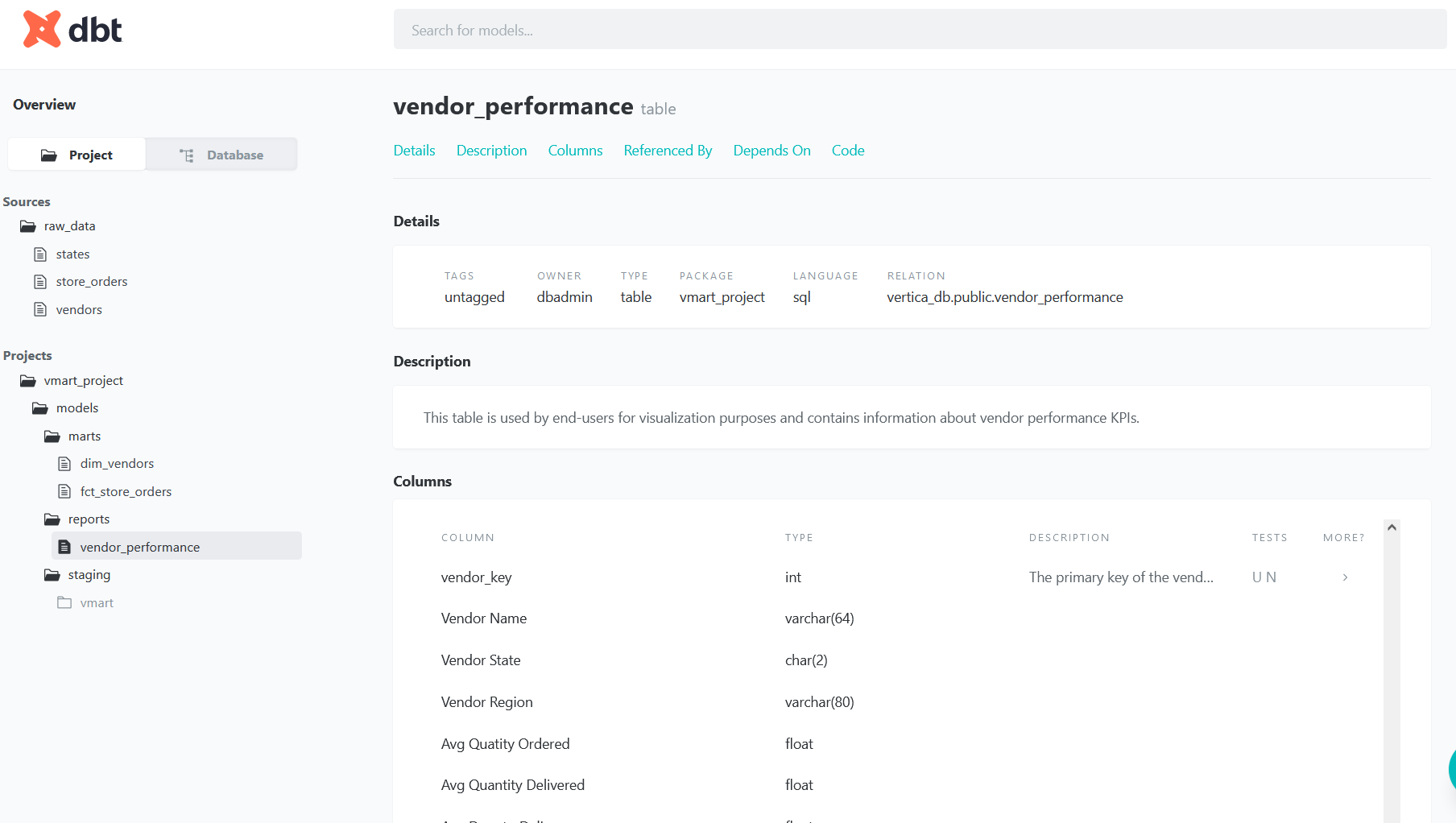
dbt docs generate and dbt docs serve. In the documentation website click on the DAG icon:

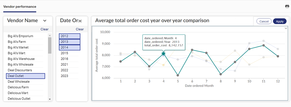
You can use any tool of your preference to connect to Vertica and visualize the data of the tables generated by dbt. In this example, we used Magellan by OpenText to create a dashboard of Vendor performance:
Summary and Conclusions
We created a comprehensive example of a data transformation pipeline that uses business logic to transform raw data into a dimension and fact table for business analytics and reporting.
Vertica + dbt constitute a powerful solution for in-database data transformation that leverages the speed of your database.
For More Information


