Vertica and Qlik Direct Discovery: A Technical Exploration
Applies to Vertica 7.2.x and earlier
About This Document
This document explores the Vertica analytic database with Qlik’s Direct Discovery feature and provides technical details and examples that demonstrate how to implement Qlik-on-Vertica using Qlik’s Direct Discovery.
The document was created with the following goals for using Qlik’s Direct Discovery with Vertica:
- Use a large fact table with fast load times and responsive dashboards
- Have Power of Gray associations for some dimensions
- Use some dimensions without associations
- Specify some dimensions without either associations or filtering functions
- Display row-level values without associations, aggregations, or filters
- To avoid synthetic keys, convert compound keys to single columns
The examples in this document were created using the Qlik Sense on Vertica QuickStart application, based on the VMart example database. Many of the concepts discussed in this document also apply to Qlik View. Both the application and example database are provided by Vertica. VMart ships with all versions of Vertica. You can find the Vertica QuickStart for Qlik Sense application on the Vertica QuickStart Examples page.
For an example of how Qlik Sense and Direct Discovery work on Vertica, view the sample video, which demonstrates a trillion-row dashboard.
Direct Discovery Overview
Traditionally, Qlik applications parse and compress source data into cache and then load the cache into memory, so all inquiries can be answered using the cache that is in-memory. Qlik’s Direct Discovery uses a hybrid model that holds only the metadata part of the application in memory but pushes queries down to the source database for processing. Users can decide how much metadata is loaded in memory by using a special syntax script named DIRECT QUERY. After the structure of the data is established, the data that is queried by Direct Discovery can merge with cached data that resides in-memory.
Qlik’s Direct Discovery holds metadata information in two tables:
- The Symbol table holds a list of distinct values for each dimension.
- The Associative table holds the relations between distinct values in different dimensions.
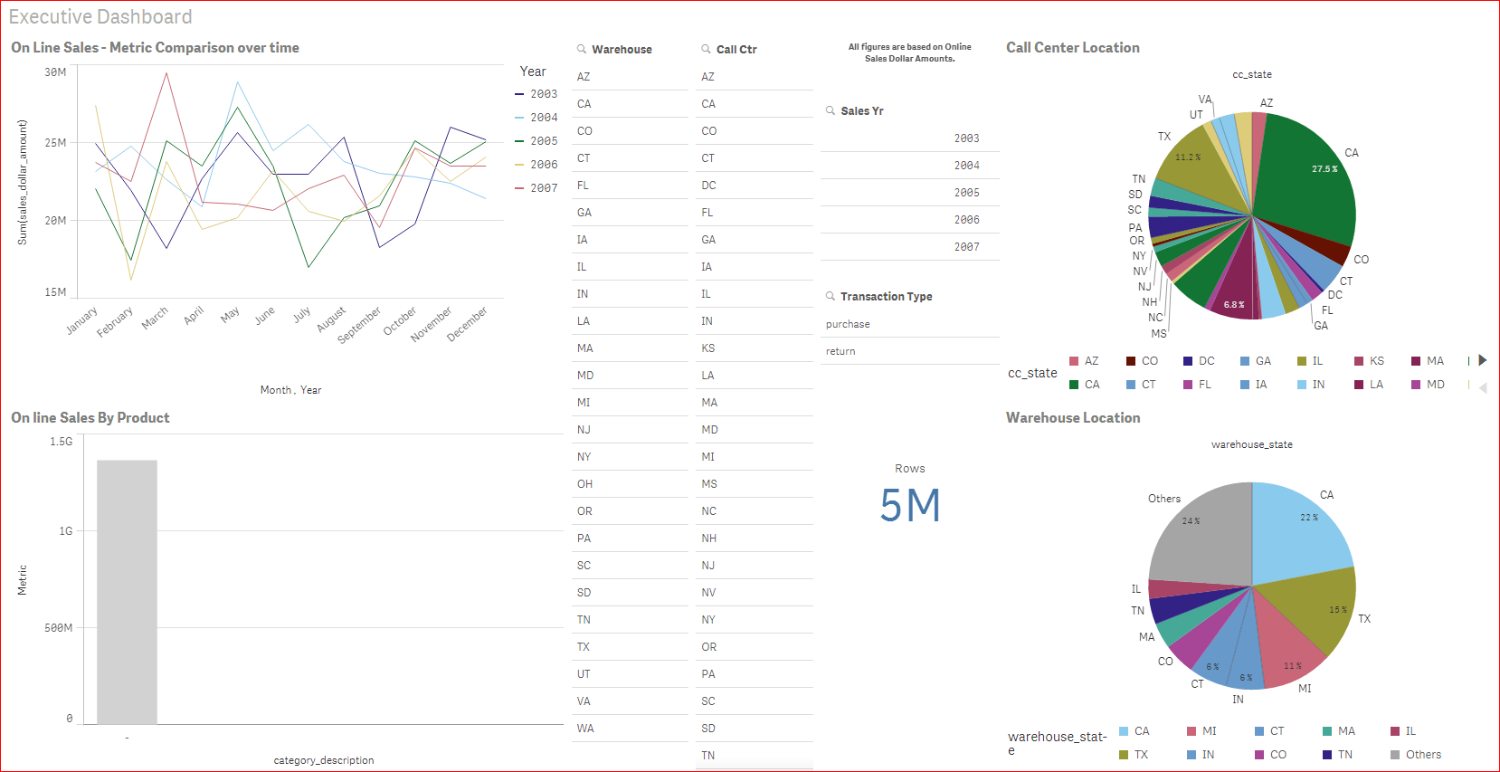
The following graphic shows an example of Qlik’s Direct Discovery Executive Dashboard. The exact appearance of your dashboard depends on your configuration. The dashboard contains various panels that show details about online sales metrics, call center information, and warehouse location information.

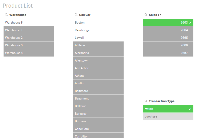
Qlik uses a color scheme to help users see which data is associated with their selections and which data is unassociated. The user’s selections are highlighted in green. Values that are related to the user’s selection are shown in white. Unrelated values are highlighted in gray. This color scheme is known as the Power of Gray and helps to color code relevant values as users make data selections.
The following graphic shows an example of associations using the Power of Gray. Note that only warehouse 5 and call centers in Boston, Cambridge, and Lowell have data for sales year 2003 and the transaction type “return”.

Direct Discovery Syntax
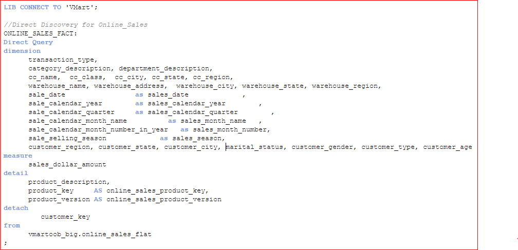
Qlik’s Direct Discovery uses its own DIRECT QUERY syntax, which is similar to a SQL SELECT statement. The main difference between the two is that the DIRECT QUERY function provides specific keywords for the different components of the query such as DIMENSION, MEASURE, DETAIL, and DETACH fields. Each one of these keywords is used to define the different sections of the Direct Discovery overall query.
The following graphic is an example script that shows the different Direct Discovery fields.

Measure Field
The fields captured under the MEASURE section do not load to a Symbol table nor to an Associative table. The MEASURE section typically holds amount fields that are aggregated by fields captured under the DIMENSION or DETACH sections. Qlik’s engine is only aware of MEASURE fields on the metadata level and does not store the actual values in memory. Be sure to put your measure fields (such as dollar amounts) under this section. Qlik automatically aggregates these values using a GROUP BY for each field under the DIMENSION section or the DETACH section that is included in the visualization.
Dimension Field
The fields under the DIMENSION section are stored in memory in both the Symbol table and the Associative table. Place values such as date, country, and gender, and so forth in the DIMENSION field. These fields are used to support the Power of Gray.
Detach Field
The fields under the DETACH section are also held in memory in the Symbol table, but they are not in the Associative table. Each detached field is its own data island. Any selection in a detached field does not change the associative data model, but does affect the direct query sent to the database. A selection in the DETACH field is included in the direct query WHERE statement. The DETACH field does not make use of the associative Power of Gray.
Detail Field
The fields under the DETAIL section are neither loaded to the Symbol table nor to the Associative table. You can see these fields in tables and the results are filtered based on selections you make on DIMENSION fields. You cannot aggregate, chart, or make a filter selection on the DETAIL field values. The primary value in DETAIL fields is that they display row-level information data in a Qlik table object.
Implementation Methods
You can use various methods to implement Qlik-on-Vertica, using in-memory load and/or Direct Discovery:
- Fact and dimension tables in-memory. Most applications are created using this approach. However, this paper does not cover the all-in-memory option because it is not suitable for big data (such as a few billion rows of fact data) and requires too much memory.
- Fact and dimension tables in Direct Discovery (regular star schema).
- BFFT (big flat fact table) in Direct Discovery. There are no dimension tables with BFFT.
- Fact tables in Direct Discovery and dimensions in memory.
- Multiple fact tables in Direct Discovery. This is not generally recommended because of complex design considerations.
- Use the Qlik API technique called “on-demand application generation”. This paper was written to understand the best way that Qlik can push as much processing as possible down to Vertica. This paper does not cover Qlik’s on-demand application generation option because this approach leverages Qlik’s Indexing Engine rather than Vertica’s processing capabilities.
Recommendations for Creating a Qlik Application Using Direct Discovery
Follow these guidelines when using Vertica with Direct Discovery:
- Use Qlik’s Direct Discovery with large fact tables. Otherwise, use the standard in-memory load option.
- Do not use multiple fact tables. If you need to report on measures from multiple facts, create separate applications.
- Qlik automatically associates your fact table with any dimension tables that have columns with the same name. If you do not want the associations done that way, rename the column in the fact or in the dimension.
- If you want the fact and dimensions to join on a column, they must have the exact same column name. The name is case sensitive.
- Direct Discovery does not support compound keys (also known as synthetic keys). If you want the fact to join a dimension on a compound key, first combine the columns into a single key in the source. For example, in VMart, two tables are joined by the compound key made up of the product_key and product_version. You could combine these two values into a combined column called prod_keyver as follows:
((product_key*100) + (product_version)) AS prod_keyver
In the Qlik load script, you must then either drop the product_key and product_version columns or rename them to prevent a compound key error.
Tuning Vertica Performance for Direct Discovery
Whenever you tune Vertica, first load some data, and run Database Designer. Then, implement Database Designer’s suggestions about the physical design of the database to load all of your data. You can also manually design and create projections or create some manually and others with the Vertica Database Designer.
Note For best results, do not manually design and create projections.
Follow these tuning suggestions to enhance the work of Database Designer:
- Create a single column projection for each column in the DIMENSION field and the DETACH field. Qlik runs a SELECT distinct on each of the fields, which populates the filter panes to support the associative Power of Gray.
- Create a projection on all of the dimension keys without any measures. Qlik frequently tries to determine what dimension keys are associated with other dimensions keys to support associations, as this example shows:
'SELECT DISTINCT "warehouse_key" FROM "big_online_sales"."online_sales_fact_medium" WHERE "transaction_type" IN ( 'return' ) AND "call_center_key" IN ( 54, 180) AND "sale_date_key" IN ( 7, 15 )'
Note If your application has a small number of measures, you can include measures in your projection. Including measures helps the projection handle the aggregation queries. However, avoid adding a large number of measures because these additions slow down the Power of Gray.
- Even though some DIMENSION fields and DETACH fields are not in filter panes, both fields can still act as filters. For example, these fields act as filters when you click on one slice on a pie chart. Direct Discovery filters all the other graphs as a result of that click. When you tune the application (either manually or using the Database Designer), be sure to consider these other dimensions and that they are used in combinations.
- Use the Vertica connection pooling feature by setting the Direct Discovery DIRECTCONNECTIONMAX parameter to a number above the default of 1. Doing so allows all graphs on a dashboard to update at the same time, rather than individually. If a Qlik Sense tab has a maximum of five visualizations, then you should set the DIRECTCONNECTIONMAX to at least five. Thus, all the visualizations can run once.
Vertica Live Aggregate Projections
In Vertica, you can use live aggregate projections (LAPs) to pre-aggregate your measures using selected dimensions. Vertica Database Designer helps you create normal projections, but not LAPs. You must design and create LAPs manually. For more information about live aggregate projections, see the Vertica documentation.
Ideally, you create a LAP based on the combination of every level of every dimension. However, this approach could result in a projection that is too large to be useful. In this case, You should create LAPs based on the combinations of dimensions that users are likely to select. Based on your specifications, the Vertica optimizer can select the correct projection to use for any query.
Vertica LAP Example
Suppose you have a big flat fact table. You want to create an application with one measure (sales_ dollar_amount) and multiple dimensions (date, month, year, customer_id, customer_type, warehouse, call_ center, product_id, product_category). Your goal is to pre-aggregate the SUM of sales_dollar_amount by the combinations of all your dimension values. However, the proposed LAP is too large because there are thousands of dates, millions of customer_ids and tens of thousands of product_ids.
Think about what your dashboard users will focus on. Create several small LAPs that provide certain subsets of dimensions. For example, you could create the following LAPs:
- One or more wide and shallow LAPs of sales_dollar_amount by year, customer_type, warehouse, call_center and product_category. This approach speeds up the exploration of all the dimensions at their top level. However, as the user dives into deeper levels, such as moving from year to quarter, this projection is not as helpful.
- Several narrow and deep LAPs of sales_dollar_amount, such as:
- By date, month, quarter, year, product_id, and product_category. This LAP focuses on products and dates.
- By year, customer_id, customer_type. This LAP focuses on the customers.
- By date, month, quarter, year, warehouse, and call_center. This LAP focuses on the warehouses and call centers by dates.
Because you created these smaller LAPs, when a user goes into a dashboard and clicks on filters related to customer attributes, the dashboard responds quickly. If another user goes into the dashboard looking for warehouse information, that user also has a fast response time. You can make many small LAPs and the Optimizer can then use them to improve speed and performance.
Creating specific, small live aggregate projections requires an understanding of how your dashboard will be used and the cardinality of each dimension and its levels. If you know users will select specific dates and specific product IDs, then have at least one LAP based on date and product_id.
Multiple Fact Tables with Direct Discovery
Qlik recommends that users pay close attention to the modeling and design of an application that uses multiple fact tables with Direct Discovery. These scenarios can result in design, maintenance, and performance issues. However, if you have a unique situation where you must use multiple fact tables, you can use other approaches to work around the issue.
Note For best results, use only single fact tables with Direct Discovery.
You must use a full outer join to join the facts together and perform the join on all columns that the facts share. You can create the full outer join in the view or create a table as a result of the join. You must also perform the join on an additional column that is always different between the tables. This additional, different column is critical because you do not want any rows of any fact tables to actually match. For example, if fact_a has ten rows and fact_b has three rows, the result of the join should be thirteen rows.
You can create the additional column by adding a column to each fact named “table_name” to each fact where the value is the name of the table. For example, fact_a would have fact_a as the value of the table_name in every row.
If both fact_a and fact_b have a column named DOB, then you must do a full outer join based on table_name and DOB. Make sure that you join on every column that fact_a and fact_b have in common, even if that means renaming the columns to be the same. If you do not rename the columns, when you do a filter pane, the filter will not affect both facts.
Note Outer joins pull null values into the mismatched columns of the results set. Thus, most aggregate functions ignore the null values and return the intended values.
Flat Fact Tables on Direct Discovery
You can create a flat fact table by degenerating all the dimension columns into the fact. The result is one wide fact table with all the columns you need for analysis. This fact table is more denormalized than a star schema. The value of the flat fact table is that you do not need to perform any joins. This approach has minimal cost because Vertica is a column-oriented database and unused columns are not accessed. You can create LAPs on a single table only. Your fact table should include all the columns you need for your LAPs.
However, loading data into the database requires more processing. Because the joins are done once, up front, instead of every time a query is submitted, you must update the big flat fact table if the dimension values change.
Known Limitations
Using Direct Discovery with Vertica has the following limitations within Qlik applications:
- IF-THEN-ELSE syntax does not work inside of aggregate functions, such as SUM. This syntax must be applied outside of the aggregation expression.
- If implemented improperly, if-then-else syntax does not work well in the application and leads to an “Internal Engine Error”.
- Users cannot clear saved filters.
- Users cannot edit a visualization or its properties if any visualization is still loading, even if you cancel the loading process. You can avoid this issue by quitting the application and restarting using the “Open without data” option.
- Quitting a running application can cause the application to freeze upon re-opening. Shut down the application and bring it back online to correct this issue.
- If a user clicks on a pane or chart, that pane refreshes or the chart updates immediately, even if a user intended to select additional values.
- Direct Discovery does not support the Vertica LIMIT syntax.
The following is a list of data type limitations for using Direct Discovery with Vertica:
- Direct Discovery displays DATE, TIME, and TIMETZ values as ‘Total’.
- Direct Discovery displays NAN values as ‘Total’.
- The LONGVAR data type causes errors.
- The LONGVARBINARY data type causes errors.
Qlik has published the following list of Qlik features that are not compatible with Direct Discovery:
- Set Analysis
- Calculated dimensions
- Direct Discovery MEASURE and DETAIL fields are not supported in Global Search
- Section access and data reduction
- Loop and Reduce
- Compound (synthetic) keys on the Direct Discovery table
- Table naming in script does not apply to the Direct table
For More Information
| For More Information About… | See… |
|---|---|
|
Vertica QuickStart for Qlik Sense |
|
|
Vertica Community Edition |
|
|
Vertica Documentation |
|
|
Big Data and Analytics Community |


