


Poisson Regression
Poisson regression is a type of generalized linear model that is commonly used to model count data, a statistical data type that describes countable quantities. Some example use cases of Poisson regression include:
-
Call center call rate prediction for workforce allocation
-
Traffic volume prediction for intelligent traffic management
-
Health insurance claim count prediction for actuarial purposes
Poisson regression assumes that the response variable has a Poisson distribution, which is a discrete probability distribution that expresses the probability of a given number of events occurring in a fixed interval of time. Three example probability mass functions for Poisson distribution are shown in the following image (source: Wikipedia, license: CC BY 3.0, via Wikimedia Commons).
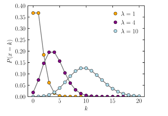
Each k in the x-axis represents a count number and the corresponding P(x=k) in the y-axis represents the probability of the actual count equaling that k. In each mass function, the parameter λ represents the expected rate of occurrence.
Dataset
In this blog post, we will use Vertica's in-DB ML functions to train and evaluate a Poisson regression model. Throughout the example, we will use the French Motor Claims Dataset, which contains the risk features and number of claims for 677,991 motor third-part liability policies observed in one accounting year. The Poisson regression model will be used to predict the frequency of claims given the set of risk features. The analyses in this blog post are inspired by [1] and [2].
First off, let's use the following commands to create and populate the table for the dataset:
CREATE TABLE claims(IDpol INT, ClaimNb INT, Exposure FLOAT, Area VARCHAR, VehPower INT, VehAge INT, DrivAge INT,
                    BonusMalus INT, VehBrand VARCHAR, VehGas VARCHAR, Density INT, Region VARCHAR);

COPY claims FROM LOCAL 'path_to_data/freMTPL2freq.csv' WITH DELIMITER ',';
Then, we can use the following command to display some sample rows in the table:
SELECT * FROM claims ORDER BY IDpol LIMIT 5;
 IDpol | ClaimNb | Exposure | Area | VehPower | VehAge | DrivAge | BonusMalus | VehBrand | VehGas  | Density | Region
-------+---------+----------+------+----------+--------+---------+------------+----------+---------+---------+--------
     1 |       1 |      0.1 | D    |        5 |      0 |      55 |         50 | B12      | Regular |    1217 | R82
     3 |       1 |     0.77 | D    |        5 |      0 |      55 |         50 | B12      | Regular |    1217 | R82
     5 |       1 |     0.75 | B    |        6 |      2 |      52 |         50 | B12      | Diesel  |      54 | R22
    10 |       1 |     0.09 | B    |        7 |      0 |      46 |         50 | B12      | Diesel  |      76 | R72
    11 |       1 |     0.84 | B    |        7 |      0 |      46 |         50 | B12      | Diesel  |      76 | R72
(5 rows)
We can see that the dataset has 12 attributes. IDpol is the policy ID and ClaimNb is the number of claims for the policy. Additionally, there are 6 numerical attributes:
-
Exposure: total exposure (i.e., policy period) in yearly units
-
VehPower: power level of the car
-
VehAge: age of the car in years
-
DrivAge: age of the (most common) driver in years
-
BonusMalus: premium bonus/penalty level between 50 and 230 (<100 is a bonus, >100 is a penalty)
-
Density: density of inhabitants per km2 in the city where the driver lives
There are 4 categorical attributes:
-
Area: area code based on inhabitant population and density
-
VehBrand: car brand
-
VehGas: diesel or regular fuel car
-
Region: regions in France
Data Preprocessing
After loading the dataset into a table, we perform some data preprocessing procedures to add helper columns and new learning features (that is, attributes).
First off, since we are going to do cross-validation for these experiments, we use the below statement to add a new column called 'Fold' that stores uniformly random Fold IDs for data split purposes.
ALTER TABLE claims ADD COLUMN Fold INT;
UPDATE claims SET Fold = FLOOR(RANDOM() * 5);  -- for 5-fold cross-validation
Then, we create a view containing the following data preprocessing steps:
-
Create a new numerical attribute called 'frequency' by dividing the claim number by the exposure for each record. The 'frequency' attribute will be the response (i.e., target) attribute.
-
Based on the lower-left figure (ref. [1]), we can see that there is a monotonic positive correlation between marginal frequency and the categorical attribute 'Area'. Therefore, we create a new numerical attribute for area called 'AreaNum' to capture this positive correlation.
-
Based on the lower-right figure (ref. [1]), the relation between marginal frequency and the numerical attribute 'VehPower' is not as simple (that is, probably a non-linear relation). We create a new categorical attribute called 'VehPowerCat' to help the learner capture such non-linear relations. This method is especially helpful for linear models, including generalized linear models such as Poisson regressors.
-
For similar reasons, we create new categorical attributes for two more numerical attributes, 'VehAge' and 'DrivAge'. The category boundaries are suggested by expert opinions in [1], which aim to achieve: (1) homogeneity within categories and (2) sufficient volume (that is, sum of exposures) of observations in each category.
-
As numerical attributes in log-linear scale are more suitable for learning Poisson regressors, we create a new numerical attribute called 'LogDensity' to contain the natural logarithmic value of 'Density'.

The following statement creates a "claims_preproc" view that has the new features from the above steps. The view also excludes old features that will not be used in the model training.
CREATE VIEW claims_preproc AS SELECT IDpol, (ClaimNb / Exposure) AS Frequency,
    (CASE Area WHEN 'A' THEN 1 WHEN 'B' THEN 2 WHEN 'C' THEN 3 WHEN 'D' THEN 4 WHEN 'E' THEN 5 ELSE 6 END) AS AreaNum,
    (CASE VehPower WHEN 4 THEN 'A' WHEN 5 THEN 'B' WHEN 6 THEN 'C' WHEN 7 THEN 'D' WHEN 8 THEN 'E' ELSE 'F' END) AS VehPowerCat,
    (CASE WHEN VehAge < 1 THEN 'A' WHEN VehAge <= 10 THEN 'B' ELSE 'C' END) AS VehAgeCat,
    (CASE WHEN DrivAge < 21 THEN 'A' WHEN DrivAge < 26 THEN 'B' WHEN DrivAge < 31 THEN 'C'
          WHEN DrivAge < 41 THEN 'D' WHEN DrivAge < 51 THEN 'E' WHEN DrivAge < 71 THEN 'F' ELSE 'G' END) AS DrivAgeCat,
    BonusMalus, VehBrand, VehGas, LN(Density) AS LogDensity, Region, Fold FROM claims;
Model Training and Evaluation
Categorical Attribute Encoding
Before training the model, we need to first encode the categorical attributes (both the original and the newly-created ones) because the Poisson regression algorithm only takes numerical features. To accomplish this, we can use one-hot encoding. The below command creates a view named "claims_encoded" that contains the original and the encoded attributes:
SELECT ONE_HOT_ENCODER_FIT('claims_encoder','claims_preproc', 'VehPowerCat, VehAgeCat, DrivAgeCat, VehBrand, VehGas, Region'
                           USING PARAMETERS output_view='claims_encoded');
Then, we can use the below command to check the attributes in the encoded view (for brevity, the records are displayed partially):
SELECT * FROM claims_encoded ORDER BY IDpol LIMIT 5;
 idpol |    frequency     | areanum | vehpowercat | VehPowerCat_1 | VehPowerCat_2 | VehPowerCat_3 | VehPowerCat_4 | VehPowerCat_5 |
-------+------------------+---------+-------------+---------------+---------------+---------------+---------------+---------------+
     1 |               10 |       4 | B           |             1 |             0 |             0 |             0 |             0 |
     3 |  1.2987012987013 |       4 | B           |             1 |             0 |             0 |             0 |             0 | ...
     5 | 1.33333333333333 |       2 | C           |             0 |             1 |             0 |             0 |             0 |
    10 | 11.1111111111111 |       2 | D           |             0 |             0 |             1 |             0 |             0 |
    11 | 1.19047619047619 |       2 | D           |             0 |             0 |             1 |             0 |             0 |
(5 rows)
It can be seen that the one-hot encoding creates a new attribute for each distinct value in a categorical attribute, and only sets one attribute to 1 among the new attributes. For example, the first record has "B" in its "VehPowerCat" attribute, which is represented by "VehPowerCat_1" in the encoding process, so only "VehPowerCat_1" is set to 1 among the encoded attributes (i.e., from "VehPowerCat_1" to "VehPowerCat_5").
Data Splitting
As mentioned above, we will conduct cross-validation (CV) to evaluate the learners. Therefore, we split the dataset according to the fold IDs. Since we conduct 5-fold CV, we use four folds as the training set and the remaining one fold as the test set. This can be realized using the below commands:
CREATE OR REPLACE VIEW claims_encoded_train AS SELECT * FROM claims_encoded WHERE Fold != 0;
CREATE OR REPLACE VIEW claims_encoded_test AS SELECT * FROM claims_encoded WHERE Fold = 0;
Note that by setting the Fold in the WHERE clauses to five different values, namely from 0 to 4, we will be able to generate the datasets for the 5 runs of the 5-fold CV.
Model Training
Now we can train our Poisson regression models. We would use the following statement to train a Poisson regressor:
\timing on
SELECT poisson_reg('m1', 'claims_encoded_train', 'Frequency', '*' USING PARAMETERS
    exclude_columns='IDpol, Frequency, VehPowerCat, VehAgeCat, DrivAgeCat, VehBrand, VehGas, Region, Fold',
    optimizer='Newton', regularization='L2', lambda=1.0, epsilon=1e-6, max_iterations=100, fit_intercept=true);
\timing off
In the above command, we have excluded multiple columns in the training process, including the ID column, the frequency and fold columns, and the columns that became obsolete during the one-hot encoding process.
As for the other training parameters, Vertica currently supports only the 'Newton' optimizer for Poisson regression. For regularization, the supported methods for Poisson regression are 'None' (default) and L2. Regularization is usually used to prevent over-fitting. Over-fitting occurs when the complexity of the model is higher than the complexity of the problem, such that the model starts to incorrectly correlate response fluctuations to the noise in the features. 'lambda' in the statement represents the regularization strength, where the larger the 'lambda' value the stronger the regularization. 'epsilon' and 'max_iteration' are cutoff parameters for model convergence determination. Finally, 'fit_intercept' is a binary flag to control whether the model should learn the intercept weight. Leaving this flag enabled usually leads to better results.
We have also turned on the timing to record the runtime of the training process.
After training the model, we can use the following command to list some detailed information about the trained model:
SELECT get_model_summary(USING PARAMETERS model_name='m1');

=======
details
=======
  predictor  |coefficient|std_err | z_value  |p_value
-------------+-----------+--------+----------+--------
  Intercept  | -1.01086  | 0.03236|-31.23629 | 0.00000
   areanum   |  0.00348  | 0.00810|  0.42962 | 0.66747
vehpowercat_1|  0.38195  | 0.00866| 44.10476 | 0.00000
vehpowercat_2|  0.45103  | 0.00886| 50.90628 | 0.00000
vehpowercat_3|  0.16870  | 0.00883| 19.09932 | 0.00000
                            ...


==============
regularization
==============
type| lambda
----+--------
 l2 | 1.00000


===========
call_string
===========
poisson_reg('public.m1', 'claims_encoded_train', '"frequency"', '*'
USING PARAMETERS exclude_columns='IDpol, Frequency, VehPowerCat, VehAgeCat, DrivAgeCat, VehBrand, VehGas, Region, Fold', optimizer='newton', epsilon=1e-06, max_iterations=100, regularization='l2', lambda=1, alpha=0.5, fit_intercept=true)

===============
Additional Info
===============
       Name       |Value
------------------+------
 iteration_count  |  5
rejected_row_count|  0
accepted_row_count|542657
The learned coefficients of the model and their significance scores are in the 'details' section (displayed partially for brevity reasons). A higher significance for a coefficient corresponds to a more important role in predicting the response. The model summary also contains information such as learning sample size and iteration count in the learning process.
Model Evaluation
We will use the Poisson deviance as the evaluation metric as shown here:
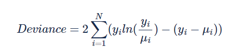
where yi and μi are the observed and predicted frequency for the i-th record and N is the number of records.
Since we conduct this deviance calculation multiple times, we create a user-defined function to perform the calculation:
CREATE FUNCTION PoissonDeviance(obs FLOAT, pred FLOAT) RETURN FLOAT
   AS BEGIN
     RETURN (CASE obs WHEN 0 THEN 2 * pred ELSE 2 * (obs * LN(obs/pred) + pred - obs) END);
   END;
For evaluation, we will calculate both the in-sample loss (i.e., training loss) and the out-of-sample loss (i.e., test loss). If the former is much lower than the latter, then the model has over-fit the training data. The training loss can be calculated using the following command (input columns to the prediction function are shown partially for brevity):
SELECT AVG(deviance) FROM (
    SELECT PoissonDeviance(obs, pred) as deviance FROM (
        SELECT Frequency AS obs,
        predict_poisson_reg(
            AreaNum,VehPowerCat_1,VehPowerCat_2,VehPowerCat_3,VehPowerCat_4, ...
        USING PARAMETERS model_name='m1') AS pred FROM claims_encoded_train
    ) AS prediction_output
) As deviance_output;
By changing the input dataset from 'claims_encoded_train' to 'claims_encoded_test', we could obtain the test loss. After repeating the process for the other 4 runs of the 5-fold CV, we get an average training loss of 2.06757 and an average test loss of 2.08162 with an average runtime of 2099.6 ms. It can be seen that the two losses are very close to each other, indicating that over-fitting has not happened in the training.
In order to get a better understanding of the Poisson regressor's performance, we can conduct another set of experiments using a more complex algorithm from Vertica, the Random Forest Regressor. We will perform the comparative experiment in the following section.
Random Forest Regression Training and Evaluation
Since the random forest model can directly intake categorical attributes, we can conduct data splitting directly on the 'claims_preproc' view. Again, by setting the fold ID in the WHERE clauses to the five possible values from 0 to 4, we can conduct the five runs of the 5-fold CV.
CREATE OR REPLACE VIEW claims_train AS SELECT * FROM claims_preproc WHERE Fold != 0;
CREATE OR REPLACE VIEW claims_test AS SELECT * FROM claims_preproc WHERE Fold = 0;
Then, we can train and evaluate a random forest model using the below commands:
\timing on
SELECT rf_regressor('m3', 'claims_train', 'Frequency', '*'
    USING PARAMETERS exclude_columns='IDpol, Frequency, Fold', max_depth=5, max_breadth=1000000000);
\timing off

SELECT AVG(deviance) FROM (SELECT PoissonDeviance(obs, pred) as deviance FROM (
        SELECT Frequency AS obs,
        predict_rf_regressor(AreaNum,VehPowerCat,VehAgeCat,DrivAgeCat,BonusMalus,VehBrand,VehGas,LogDensity,Region USING PARAMETERS model_name='m3') AS pred
        FROM claims_train) AS prediction_output) As deviance_output;

SELECT AVG(deviance) FROM (SELECT PoissonDeviance(obs, pred) as deviance FROM (
        SELECT Frequency AS obs,
        predict_rf_regressor(AreaNum,VehPowerCat,VehAgeCat,DrivAgeCat,BonusMalus,VehBrand,VehGas,LogDensity,Region USING PARAMETERS model_name='m3') AS pred
        FROM claims_test) AS prediction_output) As deviance_output;
Note that we have restricted the maximum tree depth to 5 in the training. We can conduct another two sets of experiments with tree depth set to 10 and 15 in order to choose the best model among the three versions. We've also set the maximum tree breadth to the maximum possible value so that the trees do not stop growing before reaching the set depth. The average training loss, test loss, and runtime for the three models with different max_depth are summarized in the following table:
| max_depth | training loss | test loss | runtime (ms) |
|---|---|---|---|
| 5 | 1.99674 | 2.04856 |
5897.8 |
| 10 | 1.72121 | 2.02377 |
15469.4 |
| 15 | 1.48527 | 2.02227 |
53348.2 |
We can see that increasing the max_depth parameter resulted in a decrease in training loss as well as an increase in the gap between training loss and test loss. The latter indicates that the model has probably begun to over-fit on the training data. Nevertheless, based on the 'Min CV rule', namely choosing the model that has the lowest test loss in CV, we would use the model with max_depth = 15 as our final random forest model.
Then, we can compare the final random forest model with the Poisson regressor trained in the previous section:
| model | training loss | test loss | runtime (ms) |
|---|---|---|---|
| Poisson | 2.06757 | 2.08162 |
2099.6 |
| Random forest | 1.48527 | 2.02227 |
53348.2 |
We can see that the random forest model has a test loss reduction of around 2.9%, but has a runtime much higher than that of the Poisson regressor.
Summary
In this article, we used Vertica's in-DB ML functions on the French Motor Claims dataset to load the data, preprocess and encode the attributes, and to train and evaluate a Poisson regression model using cross-validation. The experimental results showed that the Poisson regression model could achieve comparable accuracies against the more complex random forest regressor while having a much lower runtime. The trained Poisson regression model can then be used to predict claim frequencies for policy pricing purposes. As the Poisson regression model has greater explainability compared to other more complex models, it can provide more interpretable justifications for pricing decisions in the case of customer inquiries and government investigations.
References
[1] Noll, Alexander and Salzmann, Robert and Wuthrich, Mario V., Case Study: French Motor Third-Party Liability Claims (March 4, 2020). Available at SSRN: https://ssrn.com/abstract=3164764 or http://dx.doi.org/10.2139/ssrn.3164764
[2] Poisson regression and non-normal loss — scikit-learn 1.2.1 documentation

