


K-Means Clustering Using Vertica's In-Built Machine Learning Functions
This document provides step by step explanation of applying K-means on Iris Dataset using Vertica's in-built Machine Learning Functions.
K-means is a clustering algorithm that groups data into k groups such that data points in the same group are similar. Clustering algorithms are unsupervised, meaning the algorithm finds the right groups based on the features of the observations. K-means is one of the most popular clustering methods and is used in a wide variety of fields. One simple use case of k-means clustering is to identify groups of people who have similar browsing and purchasing behavior on online shopping sites such as Amazon. In this case, you could train a model to recommend products to customers based on their previous purchases and the purchase history of buyers in the same cluster.
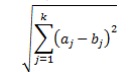
For k-means clustering, observations are often grouped based on Euclidean distance, one of the most common metrics in statistics. Euclidean distance measures the distance between a pair of samples. In a 2D space, it is simply the distance between two points:
For k-means clustering, follow these steps:
-
Randomly assign data points to clusters numbered from 1 to K cluster centroids, where K represents the number of clusters in the model.
-
For each observation, calculate the Euclidean distance between the observation and each cluster centroid. Then assign the observation to the cluster whose centroid is the closest (that is, the smallest Euclidean Distance).
-
Recompute the centroids for the newly formed clusters.
-
Repeat steps 2 and 3 until there is no change in the cluster centroids.
For a deeper dive into k-means, see the References section in this document, that links to some useful white papers.
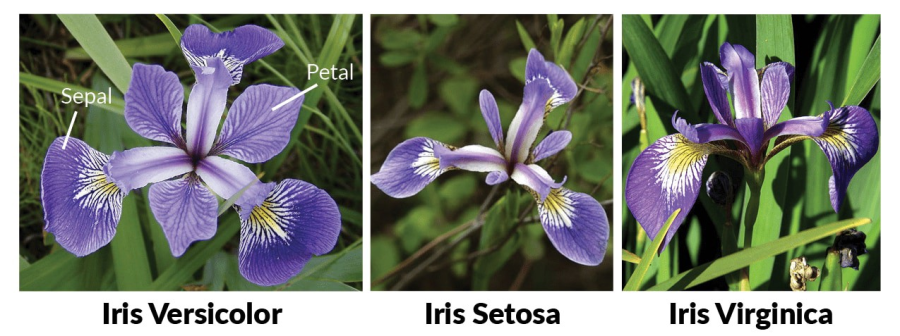
Now that we have the basics, let us apply k-means clustering on an Iris dataset using Vertica's built-in ML functions. The Iris dataset contains labeled data, but we ignore these labels during training, and only use them in the test dataset for model evaluation. This dataset contains four features (length and width of sepals and petals) for 150 samples of three species of Iris (Iris Setosa, Iris Virginica, and Iris Versicolor) [2]. One flower species is linearly separable from the other two, but the remaining two species are not linearly separable from each other [3].
In order to download the dataset, clone the Vertica Machine Learning Github repository. Within a terminal window, run the following command:
After cloning the repository, we then create a table for the training data and load the data from the iris.csv file. Once we have loaded the training data, we use the TABLESAMPLE function to create a test dataset:
mldb=> CREATE TABLE iris_train (id int, Sepal_Length float, Sepal_Width float, Petal_Length float, Petal_Width float, Species varchar(10));
CREATE TABLE

mldb=> COPY iris_train FROM LOCAL 'iris.csv' DELIMITER ',' ENCLOSED BY '"' SKIP 1;
 Rows Loaded
-------------
         150
(1 row)

mldb=> CREATE TABLE iris_test AS SELECT * FROM iris_train TABLESAMPLE(30);
CREATE TABLE
Next, delete the test data from iris_train table:
mldb=> delete from iris_train where id in (select id from iris_test);
 OUTPUT
--------
     43
(1 row)

 mldb=> commit;
COMMIT
Let us check the row counts of the train and test tables:
mldb=> select count(*) from iris_train;
 count
-------
   107
(1 row)

mldb=> select count(*) from iris_test;
 count
-------
    43
(1 row)
Data Exploration
To better understand the data, we will do a bit of data exploration. We see that we have 107 observations in the training dataset and 43 observations in the testing dataset. Based on the table definition, the dataset has four predictor variables and one target variable, Species. All four predictor variables—Sepal_Length, Sepal_Width, Petal_Length, Petal_Width—are numerical variables:
Sepal_Length: Sepal length, in centimeters
Sepal_Width: Sepal width, in centimeters
Petal_Length: Petal length, in centimeters
Petal_Width: Petal width, in centimeters
Using the above features, we will try to classify the observation into one of the following species:
We can run the SUMMARIZE_NUMCOL function to get the distribution of the features:
mldb=> SELECT SUMMARIZE_NUMCOL(Sepal_Length,Sepal_Width,Petal_Length,Petal_Width) over() from iris_train;
| COLUMN | COUNT | MEAN | STDDEV | MIN | 25% | 50% | 75% | MAX |
|---|---|---|---|---|---|---|---|---|
| Petal_Length | 107 | 3.69345794392523 | 1.79423978898708 | 1.1 | 1.5 | 4.2 | 5.1 | 6.9 |
| Petal_Width | 107 | 1.17570093457944 | 0.781005776498258 | 0.1 | 0.3 | 1.3 | 1.8 | 2.5 |
| Sepal_Length | 107 | 5.80373831775701 | 0.845401013881942 | 4.3 | 5.1 | 5.7 | 6.4 | 7.7 |
| Sepal_Width | 107 | 3.04392523364486 | 0.415768796893735 | 2.2 | 2.8 | 3 | 3.3 | 4.2 |
Data Preparation
We now prepare the data and make sure that our dataset does not contain missing values, duplicate rows, outliers, and imbalanced data.
Missing values: After checking the data, we confirm that there are no missing values for columns.
Encoding categorical columns: Since we do not have any categorical columns, there is no need to encode any columns.
Detecting outliers: Outliers are data points that greatly differ from other similar data points. Removing outliers before creating the model helps avoid possible misclassification. You can detect outliers with Vertica's DETECT_OUTLIERS function.
Normalizing the data: Normalizing the data scales numeric data from different columns down to an equivalent scale. You can normalize data with Vertica's NORMALIZE_FIT function.
The following example checks the Iris training set for any outliers:
mldb=> SELECT DETECT_OUTLIERS('iris_outliers', 'iris_train', 'Petal_Length,Petal_Width,Sepal_Length,Sepal_Width', 'robust_zscore' USING PARAMETERS outlier_threshold=3.0);
   DETECT_OUTLIERS
----------------------
 Detected 0 outliers

(1 row)
From this result, we see that there are no outliers in the training dataset.
Now, let us normalize the training dataset with NORMALIZE_FIT. This function computes normalization parameters for each of the specified columns in an input relation. The resulting model stores the normalization parameters. Next, we apply the model to the test data and create a view using APPLY_NORMALIZE:
mldb=> SELECT NORMALIZE_FIT('iris_train_normalizedfit', 'iris_train', 'Petal_Length,Petal_Width,Sepal_Length,Sepal_Width', 'robust_zscore' USING PARAMETERS output_view='iris_train_normalized');
 NORMALIZE_FIT
---------------
 Success

(1 row)

mldb=> CREATE VIEW iris_test_normalized AS SELECT APPLY_NORMALIZE (* USING PARAMETERS model_name = 'iris_train_normalizedfit') FROM iris_test;
CREATE VIEW
Correlation Matrix
We will now check how strongly the variables are associated with each other. In this example, we use the Pearson Correlation Coefficient between each pair of features. Let us use Vertica's CORR_MATRIX function:
mldb=> SELECT CORR_MATRIX("Sepal_Length", "Sepal_Width", "Petal_Length", "Petal_Width") OVER() FROM iris_train_normalized;
| variable_name_1 | variable_name_2 | corr_value | number_of_ignored_input_rows | number_of_processed_input_rows |
|---|---|---|---|---|
| Petal_Length | Petal_Width | 0.966904031755449 | 0 | 107 |
| Petal_Width | Petal_Length | 0.966904031755449 | 0 | 107 |
| Sepal_Width | Petal_Width | -0.366233624601499 | 0 | 107 |
| Petal_Width | Sepal_Width | -0.366233624601499 | 0 | 107 |
| Sepal_Width | Petal_Length | -0.421237128107181 | 0 | 107 |
| Petal_Length | Sepal_Width | -0.421237128107181 | 0 | 107 |
| Sepal_Length | Petal_Width | 0.827139137211335 | 0 | 107 |
| Petal_Width | Sepal_Length | 0.827139137211335 | 0 | 107 |
| Sepal_Length | Sepal_Width | -0.136012631154028 | 0 | 107 |
| Sepal_Width | Sepal_Length | -0.136012631154028 | 0 | 107 |
| Sepal_Length | Petal_Length | 0.882927173696874 | 0 | 107 |
| Petal_Length | Sepal_Length | 0.882927173696874 | 0 | 107 |
| Petal_Width | Petal_Width | 1 | 0 | 107 |
| Petal_Length | Petal_Length | 1 | 0 | 107 |
| Sepal_Length | Sepal_Length | 1 | 0 | 107 |
| Sepal_Width | Sepal_Width | 1 | 0 | 107 |
The correlation coefficient values are between [-1, 1], with -1 indicating a perfect negative relationship between two features and 1 indicating a perfect positive relationship between two features. Based on the above results, we see that Petal_Length and Petal_Width have a strong 0.96 positive correlation. Therefore, if the Petal_Length value increases, Petal_Width increases in a linear fashion. Sepal_Length and Petal_Length also have a strong positive correlation. Sepal_Width and Petal_Length have a moderate -0.4 negative correlation. Thus, if Septal_Width increases, Petal_Length decreases, and vice-versa.
Building K-Means Model
Let us apply k-means to the training data and build a model. We pass the id and Species columns to the exclude_columns parameter, as id is not a predictor and Species is the label:
mldb=> select kmeans('iris_model','iris_train_normalized','*',3 USING PARAMETERS max_iterations=20, output_view='myKmeansView', key_columns='id', exclude_columns='Species, id');
          kmeans
---------------------------
 Finished in 11 iterations
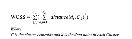
In the above example, we arbitrarily chose three clusters. To find the optimal number of clusters K, you can use the Elbow method. This method uses the Within Cluster Sum of Squared Errors (WSS) metric, which is the sum of distances between the observations and corresponding centroids for each cluster. The method calculates the WSS for various values of K and chooses the K at which WSS starts to diminish. If you draw a plot of WSS versus K, this optimal point is seen as an elbow.
If we run k-means for various values of K, say 1 through 8, we can observe the WSS scores:
| number of clusters(K) | Total WSS |
|---|---|
| 1 | 313.5278 |
| 2 | 125.1907 |
| 3 | 78.012186 |
| 4 | 60.488483 |
| 5 | 59.479389 |
| 6 | 54.267 |
| 7 | 39.831073 |
| 8 | 35.565158 |
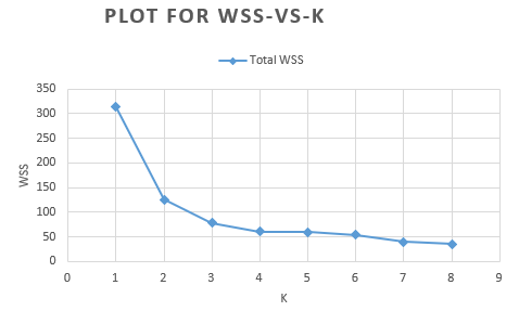
Based on this plot, we observe an elbow around K = 3 (that is, the WSS does not decrease much from K=3 to K=4). Therefore, three is the optimal value of K for this dataset and our trained model from above is best!
Let us view a summary of the 'iris_model' using the function GET_MODEL_SUMMARY:
SELECT GET_MODEL_SUMMARY (USING PARAMETERS model_name='iris_model');


=======
centers
=======
sepal_length|sepal_width|petal_length|petal_width
------------+-----------+------------+-----------
   1.25019  |  0.15670  |   0.63945  |  0.56719
  -0.80817  |  0.89932  |  -1.31773  | -0.89097
   0.03038  | -0.75349  |   0.04167  |  0.08203


=======
metrics
=======
Evaluation metrics:
     Total Sum of Squares: 313.52783
     Within-Cluster Sum of Squares:
         Cluster 0: 26.084614
         Cluster 1: 24.722264
         Cluster 2: 27.205308
     Total Within-Cluster Sum of Squares: 78.012186
     Between-Cluster Sum of Squares: 235.51565
     Between-Cluster SS / Total SS: 75.12%
We can now run APPLY_KMEANS and assign each row to a cluster center for 'iris_model':
mldb=> SELECT id, Species,APPLY_KMEANS(Sepal_Length,Sepal_Width,Petal_Length,Petal_Width USING PARAMETERS model_name='iris_model', match_by_pos='true') as predicted  FROM iris_test_normalized;

id  |  Species   | predicted
-----+------------+-----------
   4 | setosa     |         1
  15 | setosa     |         1
  20 | setosa     |         1
  23 | setosa     |         1
  25 | setosa     |         1
  38 | setosa     |         1
  54 | versicolor |         2
  56 | versicolor |         2
  59 | versicolor |         0
  63 | versicolor |         2
  75 | versicolor |         2
  99 | versicolor |         2
 103 | virginica  |         0
 127 | virginica  |         2
   3 | setosa     |         1
   6 | setosa     |         1
  16 | setosa     |         1
  21 | setosa     |         1
  61 | versicolor |         2
  71 | versicolor |         0
  73 | versicolor |         2
  78 | versicolor |         0
  93 | versicolor |         2
 122 | virginica  |         2
 139 | virginica  |         2
 142 | virginica  |         0
 144 | virginica  |         0
  27 | setosa     |         1
  37 | setosa     |         1
  65 | versicolor |         2
  66 | versicolor |         0
  67 | versicolor |         2
  74 | versicolor |         2
  86 | versicolor |         0
 104 | virginica  |         0
 111 | virginica  |         0
 112 | virginica  |         0
 116 | virginica  |         0
 123 | virginica  |         0
 125 | virginica  |         0
 132 | virginica  |         0
 135 | virginica  |         2
 138 | virginica  |         0
(43 rows)
Model Evaluation
To assist in model evaluation, we can create a table named 'iris_predicted_results' to store the original species and the species predicted by our model:
mldb=> CREATE TABLE iris_predicted_results as select * , case when predicted=0 then 'virginica' when predicted =1 then 'setosa' when predicted=2 then 'versicolor' else 'unknown' END as predicted_species  from  (SELECT id, Species, APPLY_KMEANS(Sepal_Length,Sepal_Width,Petal_Length,Petal_Width USING PARAMETERS model_name='iris_model') as predicted  FROM iris_test_normalized) foo;
CREATE TABLE
Now, let us see if our model is making accurate predictions. To do this, we create a confusion matrix, which is a matrix that compares the actual values with the target values predicted by our model:
mldb=> SELECT CONFUSION_MATRIX(species, predicted_species USING PARAMETERS num_classes=3) OVER() FROM iris_predicted_results;
 actual_class | class_index | predicted_0 | predicted_1 | predicted_2 |                   comment
--------------+-------------+-------------+-------------+-------------+---------------------------------------------
 virginica    |           0 |          11 |           4 |           0 |
 versicolor   |           1 |           5 |          11 |           0 |
 setosa       |           2 |           0 |           0 |          12 | Of 43 rows, 43 were used and 0 were ignored
(3 rows)
Based on the confusion matrix, we see that our model correctly predicted the species of 34 observations (that is, 11 correct for class 0, 11 correct for class 1, and 12 correct for class 2).
With these results, we can calculate the ERROR_RATE of the model:
mldb=> SELECT ERROR_RATE(Species,predicted_species USING PARAMETERS num_classes=3) OVER() FROM iris_predicted_results;
   class    |    error_rate     |                   comment
------------+-------------------+---------------------------------------------
 setosa     |                 0 |
 versicolor |            0.3125 |
 virginica  | 0.266666666666667 |
            | 0.209302325581395 | Of 43 rows, 43 were used and 0 were ignored
We see that our model has an average ERROR_RATE of about 0.21 across all species. Overall, the model did a pretty good job predicting flower species!

