What’s New in Vertica 9.1: Precision-Recall Curve and F1-Score Machine Learning Evaluation Functions

This blog post was authored by Ginger Ni. The precision-recall curve is a measure for evaluating binary classifiers. It is a basic measure derived from the confusion matrix. In Vertica 9.1, we provide a new machine learning evaluation function PRC() for calculating precision and recall values from the results of binary classifiers. Along with the precision and recall values, the PRC() function can calculate F1 scores as well.

Evaluate binary classifiers in Vertica

Vertica has many machine learning functions that enable users to train, score, and evaluate their machine learning models inside the Vertica database where their data is stored. Vertica supports several binary classification algorithms, such as logistic regression, SVM, and random forest. Users can train binary classifiers on the same data using different classification functions. Vertica has multiple machine learning evaluation functions that can help users evaluate their models and help them chose the best one. The PRC() evaluation function helps users pick the best binary classification model based on precision-recall or F1 score measure.

Calculate precision and recall from the confusion matrix

A dataset has two labels: positive and negative (P and N). A binary classifier predicts the dataset into two classes: predicted_positive and predicted_negative. Therefore, the dataset is separated into four outcomes: True positive(TP): actual positive and predicted positive True negative(TN): actual negative and predicted negative False positive(FP): actual negative and predicted positive False negative(FN): actual positive and predicted negative The following confusion matrix shows the four outcomes produced by a binary classifier: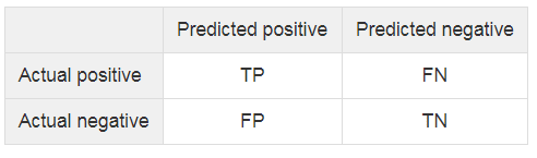 Precision is the fraction of true positive among the total predicted positive, while recall is the fraction of true positive over the total actual positive. The F1 score is the harmonic mean of the precision and recall values. Classifiers will get a high F1 score when both precision and recall are high. The F1 score provides a convenient way to evaluate binary classifiers by combining the precision and recall into a single metric.

The precision-recall curve is formed by a set of pairs of precision and recall values

A pair of precision and recall values is a point in the precision-recall space where the x-axis is recall and the y-axis is precision. A precision-recall curve is formed by connecting the adjacent precision-recall points of a classifier. We can calculate precision and recall values from multiple confusion matrices for different probability_cutoff values. For example: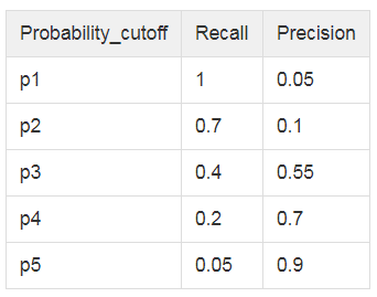 In Vertica, the PRC() function will divide the range [0, 1] into a number of equal bins. It uses the left boundaries of the bins as probability_cutoff values. For example, PRC() can divide the range [0, 1] into 5 bins, and the probability_cutoff values (p1, p2, p3, p4, p5) will be (0, 0.2, 0.4, 0.6, 0.8). The PRC() function calculates precision and recall values on multiple probability_cutoff values (which is the decision_boundary column in the output). For each probability_cutoff value, we can get a pair of precision and recall values, which is a point in the precision-recall space. By connecting those points we create a precision-recall curve.

An example of calculating precision-recall values using Vertica

Iris Data Set In this example, we are using the Iris dataset from UCI machine learning repository. It is a classification dataset with three classes: Setosa, Versicolour, and Virginica. The dataset has 150 instances and four attributes: 1. sepal length in cm, 2. sepal width in cm, 3. petal length in cm and 4. petal width in cm. To make it a binary classification dataset, we modified the class labels from Species = {Setosa, Versicolour, Virginica} to Specie_is_Setosa = {1, 0} where (Setosa = 1, Versicolour = 0, Virginica1=0). We split the dataset into a training subset and a testing subset. You can download the datasets from our GitHub repository. -- Load the data \set iris_train '''/path/to/iris_train.csv''' CREATE TABLE iris_train(id int, Sepal_Length float, Sepal_Width float, Petal_Length float, Petal_Width float, Species_is_setosa int); COPY iris_train FROM :iris_train DELIMITER ','; -- \set iris_test '''/path/to/iris_test.csv''' CREATE TABLE iris_test(id int, Sepal_Length float, Sepal_Width float, Petal_Length float, Petal_Width float, Species_is_setosa int); COPY iris_test FROM :iris_test DELIMITER ','; -- -- The training data has 90 instances SELECT count(*) FROM iris_train; count ------- 90 (1 row) -- The testing data has 60 instances SELECT count(*) FROM iris_test; count ------- 60 (1 row) Train a binary classifier using the logistic regression algorithm -- model_name = myLogisticRegModel -- input_relation = iris_train -- response_column = Species_is_setosa -- predictor_columns = Sepal_Length, Sepal_Width, Petal_Length, Petal_Width SELECT LOGISTIC_REG('myLogisticRegModel', 'iris_train', 'Species_is_setosa', 'Sepal_Length, Sepal_Width, Petal_Length, Petal_Width'); -- Please find the Syntax in Vertica Documentation Apply the logistic regression model on the testing data -- Please find the Syntax in the Vertica Documentation. SELECT id, Species_is_setosa AS target, PREDICT_LOGISTIC_REG(Sepal_Length, Sepal_Width, Petal_Length, Petal_Width USING PARAMETERS model_name='myLogisticRegModel', type = 'probability') AS probability FROM iris_test; -- You may store the result in a table CREATE TABLE scores AS SELECT id, Species_is_setosa AS target, PREDICT_LOGISTIC_REG(Sepal_Length, Sepal_Width, Petal_Length, Petal_Width USING PARAMETERS model_name='myLogisticRegModel', type = 'probability') AS probability FROM iris_test; -- SELECT * FROM scores LIMIT 5; id | target | probability ----+--------+------------------- 5 | 1 | 0.999999999999888 15 | 1 | 1 21 | 1 | 0.999999999956359 24 | 1 | 0.999999917888254 34 | 1 | 1 (5 rows)

Evaluate the logistic regression model

The machine learning evaluation function PRC() takes the target labels and the predicted probability columns as the input: Target column: the column of target labels in the binary classification data set. Probability column: the predicted probability of the response being class 1. The PRC() function divides the range [0, 1] into num_bins equally and uses the left boundaries of the bins as probability_cutoff values (which is the decision_boundary column in the output). The PRC() function will calculate precision and recall values on decision_boundary. -- The scores table is generated in the previous step. SELECT PRC(target, probability USING PARAMETERS num_bins=10, F1_Score=true) OVER() FROM scores; decision_boundary | recall | precision | f1_score | comment -------------------+--------+-------------------+----------+--------------------------------------------- 0 | 1 | 0.333333333333333 | 0.5 | 0.1 | 1 | 1 | 1 | 0.2 | 1 | 1 | 1 | 0.3 | 1 | 1 | 1 | 0.4 | 1 | 1 | 1 | 0.5 | 1 | 1 | 1 | 0.6 | 1 | 1 | 1 | 0.7 | 1 | 1 | 1 | 0.8 | 1 | 1 | 1 | 0.9 | 1 | 1 | 1 | Of 60 rows, 60 were used and 0 were ignored (10 rows) -- The scores table could from a sub-query as well. SELECT PRC(target, probability USING PARAMETERS num_bins=10, F1_Score=true) OVER() FROM (SELECT Species_is_setosa AS target, PREDICT_LOGISTIC_REG(Sepal_Length, Sepal_Width, Petal_Length, Petal_Width USING PARAMETERS model_name='myLogisticRegModel', type = 'probability') AS probability FROM iris_test) scores; The PRC() function outputs a set precision and recall pairs. In this example, the PRC() evaluation on ‘myLogisticRegModel’ presents high recall, precision and f1_score values. So ‘myLogisticRegModel’ is a pretty good binary classifier on this data set. For more information, see PRC in the Vertica documentation.