Vertica’s In-database Random Forest, Highly Scalable and Easy to Use

Arash Jalal Zadeh Fard authored this post.

Vertica has a set of machine learning tools covering a wide spectrum of advanced data analysis functionalities like data discovery, data preparation, model training, model evaluation, and model management. The goal of this blog post is to provide a hands-on example demonstrating how the built-in distributed Random Forest algorithm can be used to tackle a data science problem. We have used Vertica 9.1SP1 for running this example.

Random Forest is a popular algorithm among data scientists for training predictive models. It can be applied to both regression and classification problems. It also provides good prediction performance, and is quite robust against overfitting. The running time and memory footprint of this algorithm in R-randomForest package or Python-sklearn can be hurdles for solving Big Data problems. Our distributed implementation of Random Forest overcomes these obstacles. Training the model and managing it inside the database also relieves the overhead of transferring data into another system for analysis, and maintenance of such an extra system.

Before presenting the hands-on example, we would like to add a brief background about the Random Forest algorithm and its implementation in Vertica. Feel free to jump straight to the hands-on example if you are only interested in learning how to use it.

Under the Hood – Brief introduction to Random Forest and our implementation

Let’s refer to Random Forest as RF for short. An RF model is an ensemble of decision trees where each one is trained on a random subset of the data. Predictions based on this model are actually the aggregated predictions of all the model’s decision trees. It is noteworthy that our internally implemented decision trees are binary trees, and each of their decision nodes checks only a single condition. We have developed different functions of RF for classification and regression problems. We added RF_CLASSIFIER function in Vertica 8.1SP1, and RF_REGRESSOR in 9.0SP1.

What is random in the RF algorithm?

There are two forms of randomness in training each tree in RF:

(1) For training each tree a random subset of the data is sampled without replacement. The default sampling size is 0.632, but it can be adjusted using the sampling_size parameter.

(2) During the training of each tree, a random subset of predictors (aka features) is considered for making each split. The default number of picked predictors for RF_CLASSIFIER is the square root of the total number of predictors. Its default value for RF_REGRESSOR is one-third of the total number of predictors. This number can also be customized using the mtry parameter. The name of this parameter is inspired by the name of the similar parameter in the implementation of RF in R language. It means try m predictors each time.

What is the method for training each node of a tree?

At the time of training a decision node of a tree, the algorithm is supposed to pick the best predictor and select the best condition on that predictor to maximize the Information Gain for splitting the data to the children of that node. The information gain will be maximized when the impurity on the split data is decreased as much as possible. In simple terms, it tries to split the data into subsets such that in each one the values of response (aka target) are similar as much as possible. There are several popular methods for measuring impurity. We have used Gini Impurity in RF_CLASSIFIER and Variance Impurity in RF_REGRESSOR for this purpose. You can learn more about these concepts in the literature. Wikipedia might be a good starting point: Decision_tree_learning.

How to control the size of an RF model?

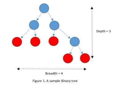
It would be wise to control the size of an RF model which is going to be trained on Big Data. A bigger RF model in size might provide a higher prediction accuracy, but its training time can grow exponentially. There are two dimensions impacting the size of an RF model: the number of trees which can be controlled by the ntree parameter and the approximate size of each individual tree in the RF model.

Decision trees can grow really huge when they are trained on Big Data without any limit. Therefore, their size should be reasonably limited in any practical solution. We have provided four parameters for this purpose: max_depth, max_breadth, min_leaf_size, and min_info_gain. The first two are easier to understand and to use. In Vertica’s implementation of RF, the depth of a tree is the maximum number of edges on the path from its root node to any leaf node. The depth of a tree with only a root node is 0. We define the breadth of a tree as the number of leaf nodes minus one. For example, the tree in Figure 1 has depth of 3 and breadth of 4. Trees in RF won’t grow beyond the values you specify for max_depth and max_breadth. Leaf size is the number of data points to be split in a decision node. There would be no further split in a node when the number of data points becomes less than min_leaf_size. There would be no split either if the information gain achieved by splitting is less than min_info_gain.

What is the impact of the number of bins on RF training?

Our distributed implementation of the RF training is inspired from the PLANET algorithm that employs histograms to summarize the information of predictors from distributed data partitions. In this approach, we need to discretize the numeric predictors. We divide the range of each numeric predictor to equal-width bins, and then replace each value with its corresponding bin index. The default number of bins is 32 and it can be changed by the nbins parameter to improve the accuracy of the discretization process.

Hands-on Example – Estimate the Price of Diamonds

We have used the Diamond dataset from the Kaggle website for this hands-on-example. The goal is to train a model for predicting the price of a diamond using its physical features. The dataset has 53940 rows and 11 columns:

• • Id: Unique identifier of each diamond in the dataset (1 — 53940)

 

• • Price: Price in US dollars ($326–$18,823)

 

• • Carat: Weight of the diamond (0.2–5.01)

 

• • Cut: Quality of the cut. Quality in increasing order Fair, Good, Very Good, Premium, Ideal

 

• • Color: Color of the diamond coded from D to J, with D being the best and J the worst

 

• • Clarity: A measurement of how clear the diamond is (I1 (worst), SI2, SI1, VS2, VS1, VVS2, VVS1, IF (best))

 

• • X: Length in mm (0–10.74)

 

• • Y: Width in mm (0–58.9)

 

• • Z: Depth in mm (0–31.8)

 

• • Depth: Total depth percentage = z / mean(x, y) = 2 * z / (x + y) (43–79)

 

• • Table: Width of top of diamond relative to widest point (43–95)

  We had used this dataset before in another blog-post to train a linear-regression model with the same goal: estimate-price-diamonds-using-vertica-machine-learning. In that blog, we also showed a few functions that you can use for data exploring. We skip those steps here, and encourage you to take a look at our older blog post. Especially, we would like you to compare the steps between training LINEAR_REG and RF_REGRESSOR models. You will notice that the latter is easier to work with. For example, you don’t need one-hot-encoder to transform the categorical predictors. Indeed, RF_REGRESSOR directly accepts both numeric and categorical (string) predictors. Also, you will notice that the RF model can provide a higher prediction accuracy in comparison.

We have used Vertica 9.1SP1 and vsql for running our SQL queries.

Loading the data to database

First, you need to download the file of the dataset on one of your Vertica nodes. You can download the file from its Kaggle page, or its copy on our GitHub page. Here, we use the one from our own page because it is compressed in GZ format and can be loaded to Vertica without uncompressing. Also, please notice that we rename columns “depth” and “table” to “diamond_depth” and “diamond_table” respectively when we create the diamond table to avoid conflict with reserved names in the database. -- setting an environmental variable for file_path \set file_path '\'/home/my_folder/diamonds.csv.gz\'' -- creating the table CREATE TABLE diamond(id int, carat float, cut varchar(10), color varchar(1), clarity varchar(10), diamond_depth float, diamond_table float, price float, x float, y float, z float); -- loading the dataset from the file to the table COPY diamond (id, carat, cut, color, clarity, diamond_depth, diamond_table, price, x, y, z) FROM LOCAL :file_path GZIP DELIMITER ',' SKIP 1 ENCLOSED BY '"'; Now, let’s randomly put aside 30% of the samples as a test dataset. We will reserve these samples unused until the very end for evaluating our trained RF model. -- creating the sample table where 30% of rows marked ‘test’ and the rest ‘train’ CREATE TABLE diamond_sample AS SELECT id, carat, cut, color, clarity, diamond_depth, diamond_table, price, x, y, z, CASE WHEN RANDOM() < 0.3 THEN 'test' ELSE 'train' END AS part FROM diamond; -- creating view for train data CREATE VIEW train_data AS SELECT id, carat, cut, color, clarity, diamond_depth, diamond_table, price, x, y, z FROM diamond_sample WHERE part = 'train'; -- creating view for test data CREATE VIEW test_data AS SELECT id, carat, cut, color, clarity, diamond_depth, diamond_table, price, x, y, z FROM diamond_sample WHERE part = 'test';

Normalizing the numeric predictors

Six predictors out of nine in our example dataset are numeric. It is usually helpful to normalize the numeric predictors. Let’s train a normalization model on train_data using the robust_zscore method. Later, we will need to apply this normalization model on test data or any other new data in order to predict the price of their diamonds. This function creates a view of the normalized train_data as well. You may investigate the content of this view if you are curious about the changes on the numeric values. -- training a normalize model on train_data and creating a view of the normalized train_data SELECT NORMALIZE_FIT ('normalize_model', 'train_data', ' carat, diamond_depth, diamond_table, x, y, z', 'robust_zscore' USING PARAMETERS output_view='normalized_train_data');

Feature selection using the RF algorithm

It is well known among data scientists that a predictive model which employs a smaller number of predictors is more reliable. In addition to the quality of the model, having fewer predictors will also shorten the training time. The RF algorithm can be used for predictor selection (aka feature selection) as well. Before training our final RF model, we train a light-weight RF model to find the most important predictors. We call this model light-weight because it has a smaller number of trees and smaller-size trees in comparison to the final model that we are going to train. -- training a light-weight RF model SELECT RF_REGRESSOR ('light_RF_model', 'normalized_train_data', 'price', '*' USING PARAMETERS exclude_columns='id, price'); We have a function in Vertica, named RF_PREDICTOR_IMPORTANCE, which calculates the importance value of the predictors in a random forest model using the Mean Decrease Impurity (MDI) approach. In a nutshell, the MDI approach uses the weighted information gain of the splits in the trees to calculate the importance values. You can find more technical details about this approach in the machine learning literature. -- finding the importance value of the predictors => SELECT RF_PREDICTOR_IMPORTANCE (USING PARAMETERS model_name='light_RF_model') ORDER BY predictor_index; predictor_index | predictor_name | importance_value ----------------+----------------+------------------ 0 | carat | 3796370.38968695 1 | cut | 14522.5775912505 2 | color | 41811.5567621371 3 | clarity | 169120.463126042 4 | diamond_depth | 16197.2323916609 5 | diamond_table | 17985.6973304553 6 | x | 1891354.92970608 7 | y | 890329.538937682 8 | z | 1960933.95168819 (9 rows) We can observe that cut, diamond_depth, and diamond_table are relatively unimportant predictors. Let’s not include them in our main RF model. We have another function in Vertica, named READ_TREE, which you can use to look at each individual trained tree or all of them in an RF model. The output of this function returns trees in Graphviz format by default. Then, you can use any Graphviz library to convert them to nice-looking graphs. This function can also return the trees in tabular format which is suitable for any further analysis. We don’t show the results of these queries here as they are quite long, but we encourage you to run them on your own database and examine the results. -- looking at an individual tree in Graphviz format SELECT READ_TREE (USING PARAMETERS model_name='light_RF_model', tree_id=0); -- looking at all trees in tabular format SELECT READ_TREE (USING PARAMETERS model_name='light_RF_model', format='tabular');

Training the predictive model

The proper settings for the ntree and max_depth parameters are not the same for different datasets and use cases. As a rule of thumb, a larger number of trees and larger-size trees in training an RF model can improve the accuracy of the final model, but it can increase the training time at the same time. In general, the default settings are good enough for Big Data problems. The dataset in this example is quite small; hence, we can set parameters higher than their default values without being worried about running time. Let’s try four different combination of the ntree and nbins parameters to study their impact on the quality of the trained model. Finally, we’ll pick the one with the best prediction performance. -- training a test predictive model with ntree=100 and nbins=100 SELECT RF_REGRESSOR ('RF_test_model1', 'normalized_train_data', 'price', 'carat, clarity, color, x, y, z' USING PARAMETERS ntree=100, max_depth=20, max_breadth=1e9, nbins = 100); -- training a test predictive model with ntree=500 and nbins=100 SELECT RF_REGRESSOR ('RF_test_model2', 'normalized_train_data', 'price', 'carat, clarity, color, x, y, z' USING PARAMETERS ntree=500, max_depth=20, max_breadth=1e9, nbins = 100); -- training a test predictive model with ntree=100 and nbins=500 SELECT RF_REGRESSOR ('RF_test_model3', 'normalized_train_data', 'price', 'carat, clarity, color, x, y, z' USING PARAMETERS ntree=100, max_depth=20, max_breadth=1e9, nbins = 500); -- training a test predictive model with ntree=500 and nbins=500 SELECT RF_REGRESSOR ('RF_test_model4', 'normalized_train_data', 'price', 'carat, clarity, color, x, y, z' USING PARAMETERS ntree=500, max_depth=20, max_breadth=1e9, nbins = 500);

Evaluating the trained models

Now, it is the time to use our test samples to evaluate the quality of our final RF model. First, we need to normalize it with the same rules that we used to normalize the train data. Here, the archived normalization model becomes handy. Let’s make a view for the normalized test data. -- normalizing the test data CREATE VIEW normalized_test_data AS SELECT APPLY_NORMALIZE (* USING PARAMETERS model_name='normalize_model') FROM test_data; Let’s store the results of our predictions on test data in a table for each trained test model. We will feed these prediction results to evaluation functions. -- predicting the price of test data using RF_test_model1 CREATE TABLE predicted_test_data1 AS SELECT price AS real_price, PREDICT_RF_REGRESSOR (carat, clarity, color, x, y, z USING PARAMETERS model_name='RF_test_model1') AS predicted_price FROM normalized_test_data; -- predicting the price of test data using RF_test_model2 CREATE TABLE predicted_test_data2 AS SELECT price AS real_price, PREDICT_RF_REGRESSOR (carat, clarity, color, x, y, z USING PARAMETERS model_name='RF_test_model2') AS predicted_price FROM normalized_test_data; -- predicting the price of test data using RF_test_model3 CREATE TABLE predicted_test_data3 AS SELECT price AS real_price, PREDICT_RF_REGRESSOR (carat, clarity, color, x, y, z USING PARAMETERS model_name='RF_test_model3') AS predicted_price FROM normalized_test_data; -- predicting the price of test data using RF_test_model4 CREATE TABLE predicted_test_data4 AS SELECT price AS real_price, PREDICT_RF_REGRESSOR (carat, clarity, color, x, y, z USING PARAMETERS model_name='RF_test_model4') AS predicted_price FROM normalized_test_data; There are several functions that we can use to evaluate the relationship between the predicted prices and the real prices in the test data: MSE (Mean Squared Error), RSQUARED, and CORR. When we compare several predictive models, lower values for MSE, and higher values for RSQUARED and CORR are preferred. Many data scientists believe that R-squared is not a valid metrics for evaluating nonlinear models; therefore, we do not calculate it for the RF models of this example. -- calculating MSE and CORR for predicted_test_data1 SELECT MSE (real_price, predicted_price) OVER() FROM predicted_test_data1; SELECT CORR (real_price, predicted_price) FROM predicted_test_data1; -- calculating MSE and CORR for predicted_test_data2 SELECT MSE (real_price, predicted_price) OVER() FROM predicted_test_data2; SELECT CORR (real_price, predicted_price) FROM predicted_test_data2; -- calculating MSE and CORR for predicted_test_data3 SELECT MSE (real_price, predicted_price) OVER() FROM predicted_test_data3; SELECT CORR (real_price, predicted_price) FROM predicted_test_data3; -- calculating MSE and CORR for predicted_test_data4 SELECT MSE (real_price, predicted_price) OVER() FROM predicted_test_data4; SELECT CORR (real_price, predicted_price) FROM predicted_test_data4; The results of the evaluations are collected in the following table. It can be observed that prediction performance of the models is not very sensitive to the ntree and nbins parameters. We encourage you to compare theses metrics with those obtained from linear regression models in our older blog. It is not surprising that RF yields better results for this dataset as it can learn a nonlinear relation between response and predictors.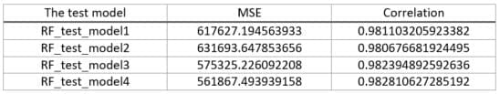



Let’s keep RF_test_model4 (which has yielded the best results) archived and drop the others. We can rename our favorite model to a more meaningful name. -- rename the selected model ALTER MODEL RF_test_model4 RENAME TO Final_RF_model; -- dropping the other models DROP MODEL RF_test_model1, RF_test_model2, RF_test_model3; -- dropping the redundant prediction tables DROP TABLE predicted_test_data1, predicted_test_data2, predicted_test_data3;

The last words

We have not printed the result of all queries here in order to save space. We encourage you to run the queries by yourself and examine each result. Please note that there is a randomness involved in separating test data in addition to the intrinsic random nature of the RF algorithm. Therefore, your final results won’t be exactly the same as those displayed here, but they should be quite close.

You might have noticed that we have created many views instead of tables in this example. Please note that views in Vertica are not materialized. That is, the query that defines a view will be executed each time the view is read. Hence, it makes sense if you cache the contents of a view which is going to be used several times in a table. If you are going to use the normalized_train_data view several times to train different models, it will be better performance-wise to store its content in a table and use that table afterwards.

The list of the archived models is available in the models table. You can drop or rename a model. In a way that is similar to how you drop or rename a table or a view. Controlling access policy of models is also similar to tables and views. You can find more about model management in our documents. What we have presented here is a small portion of what Vertica provides in its analytics toolset. Please go to our online documentation to learn more about the functions used in this example as well as other machine learning functions.