Using Vertica and HyperLogLog

This is a guest blog post co-authored by Francois Jehl and Pawel Szostek. Francois is the lead of the Analytics Data Storage team at Criteo; Pawel is a software engineer in the Analytics Data Storage team at Criteo.

Criteo is the global leader in digital performance advertising with 900B ads served in 2016. The R&D department make this possible by managing 20 000 servers in 15 datacenters, and has been intensively using Vertica for 4 years.

Today, Vertica at Criteo is deployed on more than 100 nodes and serves 200TB of analytic data to 2500 internal users every day.

Counting distinct values in a data set is a common and interesting problem in computing. There are many use cases, ranging from monitoring network equipment over genomics to computing statistics on websites.

At Criteo, we usually do not count genes, but we focus on Internet users. For those unfamiliar with us, we do online advertising, and as a consequence, we provide our clients with various metrics about their campaigns. One of these metrics is the count of distinct users that viewed, clicked, or purchased their products.

Counting Distinct Values

Let’s imagine we have a large log of all user actions. The log could look something like the following:


In our case, the log could contain billions of entries, which makes it impossible to browse the raw data. A viable solution to get the proper perspective on the data is to pre-aggregate it using time and client_id granularity. However, this can create problems for non-associative metrics, including distinct count.

Because our log is an application log, it is naturally sorted by the time of occurrence for each event. To compute the exact number of distinct users per day for each client, there are two options:

1. Use a trivial algorithm that reads in the data as-is and maintains an in-memory data structure to keep track of the count. For each value, we must consult the data structure to verify if the value was already seen. A data structure that supports an operation like this might be a hash table or a binary search tree. After the data is processed, we count the saved values and end up with a count of distinct users. This solution has a major drawback – we must retain the entire list of users seen in a day, in-memory. This will likely exceed the memory that is available.

2. Sort the data beforehand using a GROUP BY clause and then count one occurrence for each group of identical values. This is known as a sort distinct count. It has a low memory footprint, but requires that we sort the entire data set, which is a computationally complex task.

Vertica provides sorted projections, using the ORDER BY clause, which can greatly speed-up the second approach. Additionally, the SEGMENTED BY clause of projections allows us to scale out this approach on multiple nodes.

However, at a very large scale, achieving a decent query performance requires hardware investments (to scale vertically, horizontally or both). Additionally, scaling out may lead to other issues like an increase in synchronization costs during the different query planning and execution phases. In this case, we typically reduce the volume of data that we query.

Aggregating Data

Typically, we would pre-aggregate data in this scenario to solve the issue. In Vertica, we can create derivative tables that are fed by an ETL process that computes the distinct count outside the database. However, distinct count, as opposed to other aggregation functions, is non-associative. For example, if we know that client A has seen two distinct users and client B has seen three distinct users, we cannot infer the number of distinct users seen by both A and B. It is anything between 3 and 5, because there can be duplicate values.

Therefore, if we were to use distinct count in our queries, we would need to create as many aggregated tables as queries that are issues. Clearly, this would be difficult to maintain. Additionally, it could explode combinatorically if we wanted to analyze this metric among multiple axes, as many analytic applications do.

What if there was a way to store an aggregated value that was not the raw distinct count, but rather a data structure that allows us to perform associative distinct counts? That’s where HyperLogLog comes into play.

HyperLogLog to the Rescue

HyperLogLog is an algorithm that approximates distinct counts. Approximate algorithms are typically used in streaming-based systems, when you can only read the data once, and have limited memory resources.

At Criteo, we started thinking about it for the following use case: We need to provide a distinct count metric in an in-house analytical application, and we wanted to achieve sub-second response times on a very wide combination of axes. However, the desired metric did not need to be exact and a fluctuation of 1% was acceptable.

Rationale

The algorithm was originally described in [1] and has been widely used ever since. The intuition behind the paper is straightforward: if we find a hash function that converts the values you are trying to count to a binary hash, the likelihood of seeing an extreme value in those hashes is correlated to the number of distinct values you count.

For example, suppose you throw three dice. The odds of getting six three times is correlated with the number of times the dice is thrown.

HyperLogLog employs a hash function that translates any values to pseudo-random numbers, which are 64 bits long in our case. Then, it looks at the numbers from the most significant bit to the least significant bit, and counts the number of leading zeroes. As a bonus, this operation is implemented as machine instruction in most architectures.

Let’s return to the first example, which used UUIDs. We want to aggregate this table slightly. We truncate the timestamp to hours and for each UUID, we compute a 64-bit hash; we employ MurMur hash in our implementation.

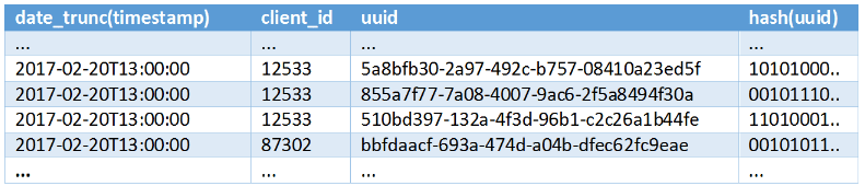
Then, for each hash, we count the leading zeroes and for each combination of (hour, client_id), we store the maximum of this value. These maxima serve as a proxy to the approximate number of distinct values seen for every client in an hour.

This approach has one major drawback: computing a single maximum for the whole dataset may lead to skews. For example, if we were unlucky, a single value with many leading zeroes would make the result unreliable. So, instead of computing one estimate, we split the stream of hashes into many streams and compute an estimate for each of them. Finally, we compute a bias-corrected harmonic mean of all the sub-estimates. This technique is called stochastic averaging.

To apply this strategy, we split the UUIDs into buckets, based on the value of the first p bits (the p is called the precision of the algorithm, because this is the main driver of accuracy). Then, when we see a number falling into a bucket, we look at the remaining 64-p bits and update the maximum held in that bucket accordingly.

After the data is processed, for every pair of (hour, client_id), we end up with arrays of 2p values (we use p bits from the hash to choose the buckets, so there will be 2p buckets). In the original paper, this array is called a synopsis. In the next section, we describe how the synopses are used to estimate cardinalities.

HyperLogLog is associative, meaning two or more synopses can be combined to create synopsis that describes the underlying data sets. This allows us to create an intermediate synopsis that summarizes a subset of rows; then we can use them to create coarse-grained aggregates. In this previous example, this means that we can aggregate client_id over hours and then combine the resulting synopses to obtain an aggregation over days.

If two or more synopses are combined, the i-th bucket in the result synopsis contains the maximum value from the i-th buckets in the input synopsis.

Raw HyperLogLog Computation

Synopses can be combined; the computation of two synopses contains maximum buckets from both. Computing a distinct count on multiple rows involves first combining all the synopses.

Then, to perform the distinct count approximation, we apply a formula on the synopsis S to obtain an estimate. The paper calls this the bias-corrected harmonic mean of the 2^M[i], where M[i] is the value stored in the i-th bucket.

We compute the mean of 2^M[i]. To minimize the effect of outliers, the researchers use the harmonic mean instead of the arithmetic one. Then, we multiply it by the square of the number of buckets and a constant alpha, determined by [1]:

The result, noted as E, is something we call the raw HyperLogLog estimate. While this estimator approaches a large count distinct with great precision, it is unable to estimate small cardinalities, which introduces a positive bias from the real cardinality. This is fairly straightforward to prove. If there are no values in the underlying data set, the synopsis M in the formula is full of zeroes. The inverted sum of 2^M[i] is equal to 1/M, and the result is a constant. Since αm is close to 0.7, that means that the result for zero values is equal to 0.7 times the number of buckets in the synopsis.

Clearly, this estimate is far from precise. However, this bias is only present for small cardinalities.

Small Cardinality Optimization

The datasets we have at Criteo are very large in most cases. However, it would be dangerous to assume that we never estimate cardinalities of smaller subsets. Thus, we have to make sure that we take care of these specific cases.

The paper’s authors were aware of this limitation and proposed to switch to another estimator, known as Hit or Linear Counting [2], when the raw estimate is small enough, and therefore burdened with the bias.

Hit Counting also uses the synopsis, but applies a simpler formula:

V represents the number of buckets in the synopsis that are set to 0. If the synopsis is empty, the logarithm of 1 is equal to 0, and the estimator returns the correct result. The intuition behind this algorithm can be approximated as the following:

The extensive demonstration can be found in [3] (in French) in section 4.3. Then, we can find the estimator for the number of balls thrown:

We use this estimator instead of the raw HyperLogLog estimate when the original value is too small by the original estimate. [1] used a constant to switch between the algorithms:

Later research done by Google [4] proved that using different values for the switch based on the synopsis size led to better results. Our implementation takes advantage of this and uses an array of constant values.

Bias Correction

While combining both algorithms demonstrated impressive precision improvements to the original algorithm, [4] emphasizes that a bias still exists for estimates too big for Linear Counting but too small for HyperLogLog to be precise enough.

The paper demonstrated effectively that this bias only exists for HLL estimates less than 5m, where m is the number of buckets in the synopsis. To correct this bias, [4] uses the k-nearest neighbor interpolation, with k being experimentally fixed to 6 – on a set of bias values determined experimentally. We made use of the arrays of interpolation points as described in [6]. This correction is applied to all raw HyperLogLog estimates below 5m.

The final algorithm includes both small cardinality optimizations, where p denotes the precision m=2p in the following:

Saving Storage Space

With this algorithm in place, now we can compute approximate distinct counts. But, like with every database engine, the performance of the algorithm is linked to the volume of data stored on disks. Our first naïve attempt was to use 8 bits to store every bucket. The rationale is pretty simple: the number of leading zeroes can go up to 63, and this value can fit in 6 bits (63 = 0b111111). Since 8 bit integers are the smallest data type able to hold such a value, we store the synopsis as arrays of 8 bit integers, even if though we knew it wasted two bits per bucket.

In our experiments we tried to see how much performance we would gain by decreasing the size of a single synopsis, which would lead to a lower memory footprint and better CPU cache utilization. We switched to an array of 6 bit buckets, as recommended by [4] and used in Redis. This means that buckets were spread across two bytes, which required some bit twiddling for serialization and deserialization to be efficient.

But what if we could reduce the storage footprint even more?

Reducing Synopsis Size Again

In practice, synopses have an interesting property – as new data is thrown into the synopsis, all the buckets tend to have similar values, as proven by [4] and [5]. This is somehow intuitive: the counts of leading zeroes in buckets of well-distributed hash values should be close to each other.

With this knowledge, we can change the serialization format and store the buckets using less than 6 bits. To this end, every serialized bucket is stored as a deviation from one of the other buckets. To do so, we changed our serialization code to switch from storing arrays:

[10,12,14,9,7,11,8,13]

Then, we serialize the synopsis as a structure like the following:

{
‘offset’ = 7,
‘values’ = [3,5,7,0,4,1,6]
}

This change allowed us to store buckets in 5 bits, like some similar implementations, or even go down to 4 bits, like in Metamarket’s Druid or Facebook Presto. This optimization brings a risk of clipping a value if it doesn’t fit into 4 bits. For instance, if one of the buckets equals 0, the reference offset value would be also 0 and hence the maximal value fitting in a bucket would be 15 (as 2^4-1 = 15). Any value beyond 15 would be trimmed to 15, leading to accuracy loss. However, as was proved in [5], this situation is very unlikely. In our tests we noticed some cases of clipping, but its impact on the overall result was negligible.

Integrating in Vertica

We implemented two User-Defined Aggregate Functions (UDAF) using Vertica’s SDK. These functions operate on a set of values and return a single value. There were two constraints:

• The functions must be developed in C++
• They only run in non-fenced mode (i.e., only within the main Vertica process)

Classes and Calls to Implement

To define a UDAF, a developer must first extend the base AggregateFunction class, and provide the following calls:
• initAggregate(ServerInterface &srvInterface, IntermediateAggs &aggs)
• aggregate(ServerInterface &srvInterface, BlockReader &argReader, IntermediateAggs &aggs)
• combine(ServerInterface &srvInterface, IntermediateAggs &aggs, MultipleIntermediateAggs &aggsOther)
• terminate(ServerInterface &srvInterface, BlockWriter &resWriter, IntermediateAggs &aggs)

InitAggregate

This is the initialization call, where member variables and starting values for the aggregate should be set. It can be called multiple times by the engine in a single execution plan. Because it will get called from many threads on many machines, it should be idempotent.

The first value for the computation was set in an IntermediateAggs – a wrapper around a VerticaBlock – an in-memory block of data that can contain multiple columns, so that the calls that follow can start to operate on it.

In our case, we create an empty synopsis and serialize it in the IntermediateAggs.

Aggregate

Aggregate is the main function in the Aggregate function. It is given a BlockReader – an iterator of rows within a single block – and will read all the values provided by the iterator. It performs the actual aggregation based on the business logic. The aggregate also performs the aggregation and outputs a single value in an IntermediateAggs block.

The number of calls of the aggregate function depends on two things:
• The sort order of the GROUP BY key within the projection used by the query
• The existence of the minimizeCallCount hint in the UDAF factory

To better understand, let’s look at an example with a simple (key,value) projection, where we call the function f() on the value column, aggregated by key. The UDAF performs a call to aggregate() for every group of keys read sequentially:

Combine

After looking at the table above, we can guess that the combine function is in charge of performing the last aggregation operation of the various aggregate() calls on the same key. It is given an iterator of IntermediateAggs, called MultipleIntermediateAggs, that it must aggregate within a single IntermediateAggs block. Generally, the same business logic is used in both functions.

Terminate

The last function gets called for every key and outputs the data in a BlockWriter. It reads the single block of data and writes it with the help of the BlockWriter. The implementation can be as simple as the following: const vfloat max = aggs.getFloatRef(0); resWriter.setFloat(max);

AggregateFunctionFactory Class

An AggregateFunctionFactory must be created and registered. It provides a set of methods used to declare:
• The function parameters
• The function return types
• The structure of the IntermediateAggs block that the AggregateFunction needs

Batching Rows Together

An essential detail to remember when implementing the UDAF is the _minimizeCallCount hint. This hint, which was added to the UDAF as a function parameter, tells Vertica to batch the rows together to reduce the number of calls to the aggregate() function. If you do not use this hint, Vertica creates an aggregate for every row and then combines the aggregates. This behavior is highly inefficient because it creates a large number of nearly empty synopses. You can view the logs by using SrvInterface.log().

To circumvent this, you must define a hint parameter from inside the factory: virtual void getParameterType(ServerInterface &srvInterface, SizedColumnTypes & parameterTypes) { parameterTypes.addInt("_minimizeCallCount"); }

Building and Registering Your UDAF

A makefile is provided in the Vertica UDx examples on GitHub. The makefile builds two classes against the Vertica SDK that are installed as part of the Vertica server installation package.

After a *.so library is built, registering occurs within the database, with simple CREATE statements: => CREATE LIBRARY MyLib AS ‘mylib.so’; => CREATE AGGREGATE FUNCTION MyFunction AS LANGUAGE 'C++' NAME ‘MyFunction’ LIBRARY MyLib; After it is granted to the users, it can be used in any SQL query.

Using HyperLogLog in Hive

Hive is a Java-based SQL interface for HDFS that provides both a semantic layer and a SQL dialect to generate jobs that operate on data stored in HDFS, using various execution engines.

It’s the most commonly used ETL technology at Criteo: our analysts have created hundreds of Hive jobs to run daily. The data extracted and transformed by them is later loaded into Vertica using vsql batch insertions within Hadoop streaming jobs.

To use C++ code in a Java-based system like Hive, we use Java Native Access from within the Hive SDK to create Hive UDFs that use non-managed code underneath. Since our Hadoop nodes are configured so they don’t allow significant volumnes of memory to be allocated outside of JVM (and this happens when running native code from Hive), we were forced to implement a Hive UDF that serializes and deserializes for each number added to the synopsis. This inefficiency however has no significant impact on execution time of our Hive jobs.

That allows us to perform the synopsis creation, which is an intensive operation, on the Hadoop side, using the same business logic that is later used in Vertica to operate on those synopses and perform the actual distinct count.

Studies

We tested our UDAF against two existing HyperLogLog implementations at Criteo: the existing APPROXIMATE_DISTINCT_COUNT in Vertica, and Druid.

Comparison with Vertica APPROXIMATE_DISTINCT_COUNT

We imported 300 million rows of a click log sample on a 3 node cluster, running Vertica 7.2 on CentOS 7.2 using the following hardware:
• 2 x Intel Xeon E5-2630L v3 @1.8GHz (16 cores + 16HT)
• 256 GB DDR 4 @ 1886MHz
• RAID0 on HP P440 controller with 6 x 400 GB SSD

In our studies we were launching a simple distinct count call grouped by a key.

Because Vertica uses a constant synopsis size of 49154GB and constant precision, there was not much tuning to apply. In the following plots we show results for the only precision value offered by the available implementation, which is 16 judging by the synopsis size.

Our implementation is approximately 50 times faster for 10 bits of precision (bits used to create the buckets, which means buckets from 0b0000000000 to 0b1111111111 = 1024 buckets). We’re still more than three times faster, using 32 times more buckets.

This is especially interesting when we look at the precision:

We notice that with 13 bits of precision we achieve a similar mean error, and it is still 10 times faster. The 2% mean error is considered acceptable for this type of computation.

Comparison with Druid

We generated a test data set in Hadoop Hive composed of random integers. Then, we registered two Hive UDFs, one containing our HLL implementation and one containing Druid’s implementation. Then, we applied both implementations to the data. We varied the cardinality to see if it had any impact on the precision. We used the following settings for the implementation:
• 12 bits for bucketing
• 6 bits for each bucket

Even with a very modest precision (12 bits), our implementation was most precise in most cases than Druid.

Conclusion

In this post, we demonstrated that HyperLogLog allows you to implement very precise approximate distinct counts in Vertica, with the help of the SDK. Our implementation can also be used in Java-based engines, such as Hive, to perform CPU intensive operations, such as synopsis generation.

The code is open source and can be pulled from Criteo GitHub.

References

[1] P. Flajolet, E. Fusy, O. Gandouet et F. Meunier, HyperLogLog: the analysis of a near-optimal cardinality estimation algorithm, 2007.
[2] K. Y. Whang, B. Vander-Zanden et H. Taylor, A Linear-Time Probabilistic Counting Algorithm for Database Application, 1990.
[3] M. Durand, Combinatoire analytique et algorithmique des ensembles de données, 2004. [4] S. Heule, M. Nunkesser et A. Hall, HyperLogLog in Practice: Algorithmic Engineering of a State of The Art Cardinality Estimation Algorithm.
[5] N. Ray et F. Yang, How We Scaled HyperLogLog: Three Real-World Optimizations.
[6] S. Heule, M. Nunkesser, and A. Hall, Appendix to HyperLogLog in Practice: Algorithmic Engineering of a State of the Art Cardinality Estimation Algorithm.