


For those who have read my previous blog postings, attended one of our Big Data & Machine Learning Meetups, or have met me at one of the many trade shows or conferences over the years, you will be all too aware of my love for tracking aircraft using a Raspberry Pi, Kafka and Vertica.
For those who are not aware, a Raspberry Pi (RPI) is a credit-card sized computer, to which I connect a USB radio receiver and antenna, and by means of some open-source software and a home-built Extract, Transform and Load (ETL) application, have a “radar” that can capture aircraft location data in the form of ADS-B radio signals from aircraft transponders. If you want to read more about this, head over to one of my blog posts on Vertica.com.
I would often refer to the three primary radars we have in Geneva, New York’s JFK and Pennard – and go on to explain that Pennard is the small village in South Wales where I live and work.
It is these three primary radars that would typically capture 100m messages per day from aircraft in their 200-300K km2 catchment area, and provide for some great demonstrations on what Vertica can do with data – especially when there’s lots of it, such as the 50bn records captured since I started this project.
Roaming Radars
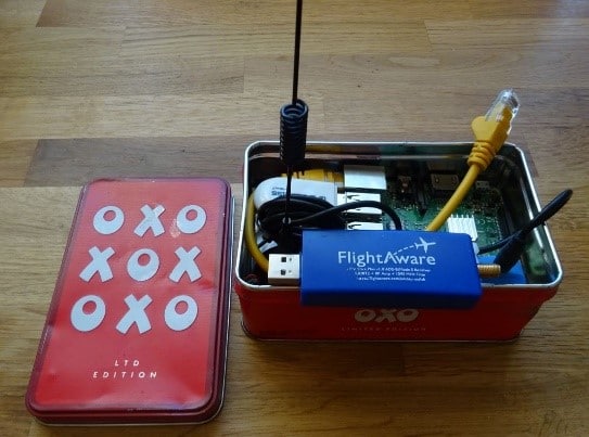
In addition to the three static radars, I also have a small number of others that would travel in an OXO tin with me when attending trade shows, conferences and even going on holiday (just don’t tell the wife ;-)).
However, these “roaming radars” presented me with a small problem. When I power up the RPI in whatever far flung location I was now in, I would immediately have to login and change one of the ETL parameters to indicate my current location with a carefully calculated latitude and longitude, and although not quite so important, the altitude of the “radar”.
RPI GPS
In keeping with how this flight-tracking project came into being, I wanted to resolve this radar-location problem with something that was both simple to achieve, and keeping the budget low.
Reverting to my research into ADS-B, it didn’t take long to work out that if aircraft can determine their position via GPS satellites, then why can’t I?
Starting my research with a Google search for “Aircraft GPS Receivers”, I soon came across options such as the Avidyne IFD550 at a mere £19,800. With the Raspberry PI coming in at ~£35, and a very limited budget, there’s clearly no way I am going to be able to justify one of these.
I even turned the Sort By Price option upside down; Low-to-High. That didn’t help much, as the lowest cost receiver was the Garmin G5 at just over £2,000.
Time to try a different tack. Just as searching for “luxury”, “premium” or “yacht” would typically attract high-end, high-cost products or services, I guessed that by including “aircraft” would have a similar effect – after all an Airbus A340-300 could set you back well over £200,000,000. Let’s see what happens if I just search for “GPS Receivers”.
That’s more like it. Far more options, with units from £100 down to a mere £5.
Scrolling through the hundreds of options out there, I decided to refine my search to include USB. After all, I wanted to be able to connect this to the RPI, and although I had done some experimenting with the 40x GPIO pins on the RPI, I was looking for something easier to setup and configure.
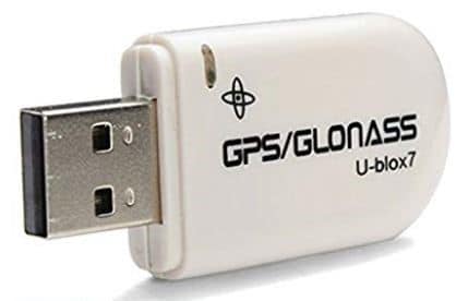
I then spotted just what I was looking for. A USB VK-172 USB GPS Receiver made by a company called u-Blox – with headquarters in Switzerland. After reading all the blurb, great reviews about the product, and the excellent u-Blox website, at £5 each, I ordered 10 of them! OK, I’d have to wait a couple of weeks for them to arrive from China – but as the UK-resellers were asking anything up to £20 each, I decided the wait was worthwhile. After all, this is money coming out of my own pocket, and I had already decided I would like to give some of these away to friends and colleagues (something that did actually happen about 12 months later – subject of another blog).
GPS
With a couple of weeks to wait until they arrived, time to understand a little more about GPS, and as I was soon to discover, other systems such as Galileo and Glonass.
Thanks to my friend Wikipedia, I found a brief introduction to GPS (summarised here):
The GPS concept is based on time, and the known position of satellites. The satellites carry very stable atomic clocks that are synchronized with one another and with ground clocks. Any drift from true time maintained on the ground is corrected daily. In the same manner, the satellite locations are known with great precision.
Each GPS satellite continuously transmits a radio signal containing the current time and data about its position. Since the speed of radio waves is constant and independent of the satellite speed, the time delay between when the satellite transmits a signal and the receiver receives it, is proportional to the distance from the satellite to the receiver. A GPS receiver monitors multiple satellites and solves equations to determine the precise position of the receiver and its deviation from true time. At a minimum, four satellites must be in view of the receiver for it to compute four unknown quantities (three position coordinates and clock deviation from satellite time).
As of December 2018, 73 GPS satellites have been launched. 31 remain operational, 9 are in reserve, 1 is being tested, 30 have been retired and 2 were lost during their launch.
National Marine Electronics Association
My research often referred to what I had been calling a “GPS Receiver” as “Global Navigation Satellite System (GNSS) Receivers”.
Either way, according to the literature I had fumbled across, the data presented by these devices conforms to a standard defined by the National Marine Electronics Association (NMEA). There are many references to the work of this organisation, but when I found that it was going to set me back $4,000 just to get the documentation which details this standard, that limited budget was clearly not going to stretch to that.
Thankfully, I found some personal research published by Dale DePriest which provided just what I needed. However, as a number of the links in Dale’s research had already “disappeared”, just in case his did too, I immediately saved the 20-page document as a PDF.
In summary, the standard defined by the NMEA, enables various pieces of marine electronic equipment and computers to communicate with each other. Not surprisingly, ships/boats also need to know where in the world they are, and especially those super tankers that they want to avoid bumping in to. As such, they too make use of GPS for positional awareness.
It would seem that this standard has since been adopted by other, non-marine applications.
Sentences
Devices adopting the NMEA standard, communicate via self-contained, independent sentences – of which there are many sentence structures. Each of these is identified by their own two-character categorisation prefix. For GPS, this prefix is “GP”, and thus, I will ignore any other categories.
The GP prefix is then followed by a 3-character sequence which in turn defines the sentence contents. As I was soon to discover, although there are approximately 30 different GP-type sentences, I would come across just 7 of them. These will be discussed shortly.
Each sentence begins with a ‘$’ and ends with a carriage return/line feed and can be no longer than 80 characters, with fields separated by a comma.
As clear as mud!
I have a plan
Whilst patiently awaiting for the GNSS receivers to arrive, I was already well on my way to understanding what they might be able to do and about how I would deploy them.
Not an expert in the field, but I knew enough to be dangerous :-).
Anticipating someone asking how I was planning on implementing this project, I thought I would use Visio to draw out what I had in my mind. I then discovered, that although I previously had access to Visio that too had disappeared. Thus I resorted to pencil and paper – in fact the pencil came out of the colouring box of my then 3 year-old Granddaughter, Lola!
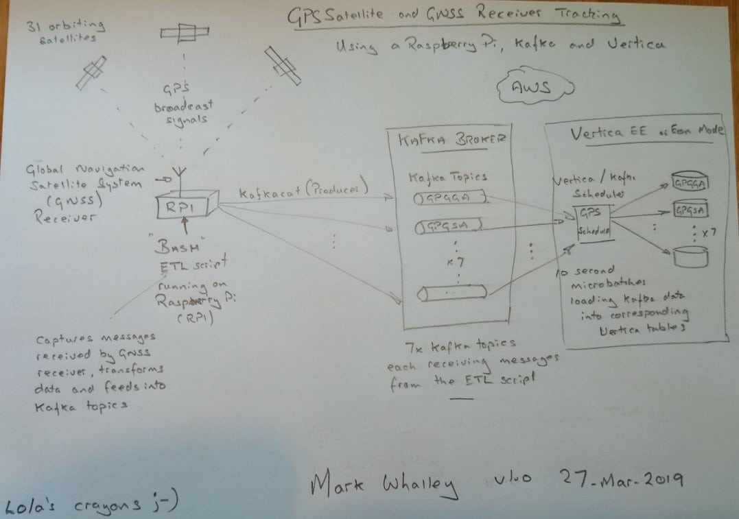
In a similar way to how I had set up the live flight tracking project, the GNSS Receiver would be attached to a RPI. I would write an ETL application using my favourite Bash shell, to capture these NMEA messages, and perform whatever transformation that needed to be done. Using Kafkacat’s “producer” option, I would feed these separate sentence categories into their own Kafka topics.
I also opted for an 8th topic to capture any “stray” NMEA messages. This subsequently proved to be a good move, for when I purchased a further, more advanced GNSS Receiver, I discovered it had slightly different two-character sentence prefixes. This later GNSS Receiver is capable of handling GPS, Glonass and Galileo satellite data with GP, GL and GA prefixes respectively.
GNSS Receivers have landed
Unlike so many of the other parcel and packet delivery services, it seems rather ironic that I was unable to track the package of 10x GNSS Receivers coming from China. However, they did in due course arrive, and now to start experimenting.
On connecting a GNSS Receiver to the RPI, it presents itself as a serial device called “ttyACM0” under /dev.
Logged in as root (or from a user who has sudo permissions), I ran the following:
sudo cat /dev/ttyACM0 | grep –v ^$
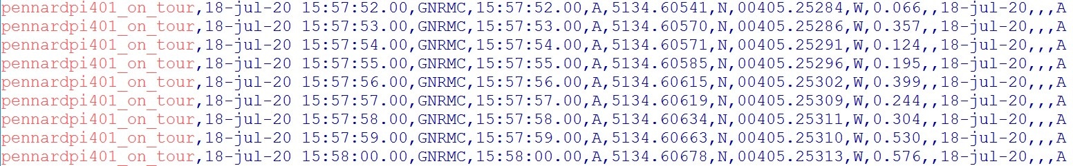
Immediately, it started to stream data similar to the following (noting here I am showing the newer GNSS Receiver with its support for GPS, Glonass and Galileo):
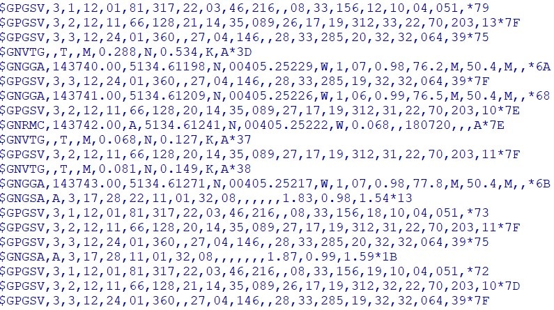
All starting to look promising, as I am seeing just what I had been reading about. Streams of messages, prefixed with a $ and terminated with CR/LF. The fields are comma-separated and are categorized by the 5-character message id. As expected, some of these showing GP (for GPS) and GN (Glonass) followed by the 3-character identifier.
I remember reading about “GSV”, and that this reports the number of satellites in view. Having no idea how many satellites would be in view at any one point, I knew there were just over 30 circumnavigating the earth.
It took a little working out, but I soon found that the reason there are multiple grouped GSV sentences, is due to the limit of 80 characters per sentence, as defined by the NMEA standard. So, looking here at a group of 3x GSV sentences, I found that the 4th field (here showing “12”), implies I am currently seeing 12 satellites – not bad for a £5 receiver sitting on my desk with limited view of the sky.

As the details of all 12 satellites cannot be reported in a single sentence, they have to be split into separate sentences. Thus the 2nd field (all reported here as “3”) indicates how many sentences I need to receive to get the full set of 12 satellites. The 3rd field (“1”, “2” then “3”) tells me which of the 3 sentences I am currently receiving.
Looking further into these sentences, I find that each sentence can report up to 4 satellites at a time, with each one providing:
- Satellite PRN number
- Elevation in degrees
- Azimuth in degrees
- SNR (Signal to Noise Ratio – or signal strength) – the higher, the better.
Of course, I then had to try and work out what all these new terms meant 😉
Thankfully, Wikipedia provided me with details of PRN (Pseudo-Random Noise!).
I won’t go through all the sentence classifications here, other than to say, it looks as though I am able to pick the following ones up with these GNSS Receivers:
- GGA Global positioning system fix data
- GLL Global positioning latitude/longitude
- GSA GPS DOP and active satellites
- GSV GPS satellites in view
- RMC Recommended minimum specific GPS/Transit data
- VTG Track made good and ground speed
- TXT Must admit to never really working out what this one is 😉
Time to start coding
Armed with my list of sentence categories, and some details of what each of these contain from Dale DePriest’s web site (mentioned above), and a further useful site from Glenn Baddeley (which I have also saved as a PDF just in case this too disappears ;-)), I am now able to start coding the ETL application. Among other transformation tasks, I decided that one of these is to present the satellites in view (GSV) sentences, which as I discovered can each have 1, 2, 3 or 4 satellites reported in multiple grouped sentences, as separate satellite records in my Vertica database.
1,600 lines of code later, and having defined 8x Kafka Topics (7x for the “known” sentences, and one called GPUNK to capture any “UNKown” ones), I can now see if data is being sent (produced) into my Kafka Broker.
Kafkacat – Consumer
Using that really useful kafkacat tool in its -C (Consume) mode, I point it at some of the topics to see what’s landing in there.
Starting with that troublesome GSV set of sentences, here I can see that when, for example, I have 12 satellites in view, I end up with 12 records in Kafka (noting that the signal strength field is often reported as NULL):
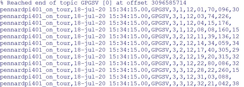
For the more observant, you may have spotted the offset of this topic – currently reporting just over 3 billion!

Looking at the VTG (Track made good and ground speed) sentences in Kafka, the “track” is shown as NULL (this is the field after “GNVTG”). The “T” indicating that the track is relative to true north. The “0.035” / “N” and “0.064” / “K” indicate the speed over the ground in kNots and Kilometres/hour.
I initially found this rather strange, as the GNSS Receiver was just sitting on my desk – not moving at all. However, on investigating further, GPS is not 100% accurate, and a speed of 0.064 km/hr is so small, it’s hardly worth worrying about.
And if it’s not moving, the track (or direction of travel) would be, as expect NULL.
One of my other challenges, is that unlike the flight tracking application, where each “message” had a time stamp appended, the NMEA specification has just one sentence that reports the timestamp. This being the RMC sentence.

As I want to have all my Kafka topics include the timestamp, I have to wait until I receive the first RMC sentence before I can start publishing the other sentences to Kafka.
Thankfully, as the GNSS Receiver pushes out one of these every second, I do not have to wait long until I know what time it is 😉
Vertica / Kafka Scheduler
Getting this far has been really great, but as we know, just publishing messages into a series of Kafka topics is a total waste of time, unless we are going to do something with it.
The obvious choice if we want to do something really useful, at great speed, and with a toolbox that knows no bounds, is to stream this data into our Vertica database!
With a really simple-to-use set of tools, I can quickly and easily setup what Vertica calls a Kafka Scheduler. With this, I introduce my Kafka broker and its topics (sources) to Vertica. I declare the tables (destinations) I want this streaming data to land in Vertica, and provide details of what the data looks like – in this case as simple as stating it is comma-separated (CSV). Finally, I tell Vertica how frequently I want it to reach out to Kafka to load any new messages waiting to be processed. I set this to 10 seconds, but like so many other aspects of Vertica, it is totally flexible and configurable to meet your needs.
There are a number of other things we can configure (such as Resource Pools), but no need to worry about these just now.
With the Kafka Scheduler defined, we can hit the “launch” button, and get that data continuously streaming into Vertica.
There’s a whole raft of tools in Vertica we can use to monitor what’s going on, but for me, I like to head over to Vertica’s Management Console (MC).
From here, we can see at a glance the health of our Kafka Scheduler, and that it is, as expected, loading data in those 10-second micro batches.
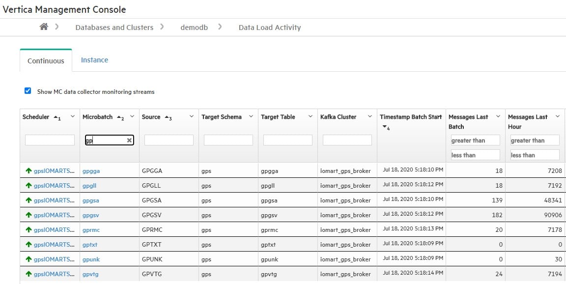
In the snippet above, I can see my 8x Kafka topics (e.g. GPGSV) feeding into their corresponding Vertica tables (gpgsv), and that in the last 10-second micro batch, how many messages it has processed (182 for GSV), and how many it has processed in the last hour (90k for GSV).
All-in-all, everything looks fine, and was so simple to setup – even I managed to do it 😉
In conclusion
What I had originally set out to achieve, was to find a simple (and cheap) solution for determining the GPS coordinates (longitude, latitude and altitude) of my portable Raspberry Pi when it traveled with me to far-flung destinations. This would mean I no longer had to manually work out my coordinates and update the parameters for the Flight Tracking Project.
Now, I know, down to the second, exactly where my Raspberry Pi is.
Problem solved 🙂
However, what I then realised, was that if I can track the position of the RPI when it arrived at that eventual destination, what was preventing me from capturing the data whilst the RPI was en-route to that destination?
Thus a whole new use case for this GPS data started to emerge.
The truly “portable” RPI (with extra bells ‘n whistles)
If I can find a way of powering the RPI whilst it is travelling, and to feed the data it captures directly to the Kafka Broker, then I can do some live RPI tracking (as well as Flight Tracking).
Thus the portable RPI was moved out of its OXO tin into a purpose-built RPI tower (there have now been several variations on this!).
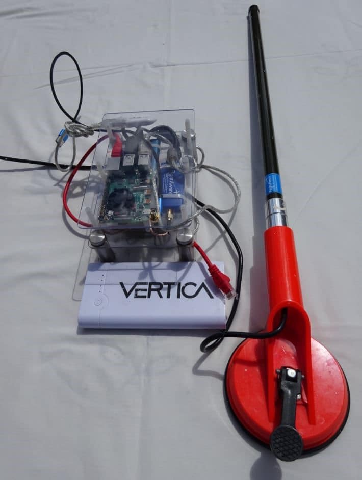
Add to this a hefty 20,000 mHa 5v power pack, embossed with “Vertica” – so literally “Powered by Vertica”. That amount of energy is enough to keep the RPI alive for several days.
To increase its storage capacity from the 16GB SD card, I added a 500GB SSD drive. Far more than I needed, but heck, I think of how much I saved by not buying that Avidyne Aircraft GPS Receiver at ~£20k, or the NMEA documentation at $4k!
I built the case from offcuts of clear sheeting and used stainless steel off-wall picture frame mounts as pillars. Far better than some of the plastic alternatives I had used in earlier models.
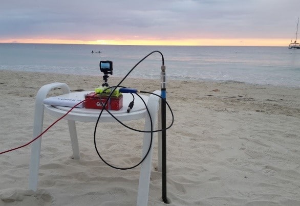
I had already upgraded the original ADS-B receiver for one which had a built-in RF Amplifier and 1090MHz Filter, and opted for the much longer 1090 MHz antenna (itself costing more than the Raspberry Pi computer to which it is attached). A challenge I was often faced with when taking this rig to trade shows and events, is where to place the antenna. When I used the smaller antennae, it was not a problem. But a 0.5m stick and its cable were always getting in the way, or falling off podiums. Thanks to a local hardware store, I found the perfect solution.

A double-cup suction lifter, perfect for safely lifting large panes of glass, sheet material and marble.
I worked out, that if I cut the hollow handle in half, the base of the antenna would fit snugly inside, with the cable protruding from the base of the handle. Then I could use the now single-cup to “stick” to a window or marble surface. It worked a treat 🙂
There are of course still lots of cable ties as with the earlier incarnations of this, but it’s now starting to look far more robust and professional – even if it’s still a Raspberry Pi at the heart.
Though to be quite honest, having seen that a new Raspberry Pi 4 had been brought out, with even more memory (at the time going up to 4GB), and with USB-3 and 2 (compared to the previous USB-2), two 4k HDMI ports, a more powerful processor (Broadcom BCM2711 Quad Core Cortex-A72) and a USB-C power supply connector, I just HAD to have one!
Not that I needed the extra RAM (after all, this project first started on the 0.5GB RAM RPI), and I don’t need two 4k HDMI ports – as the RPI is headless for most of its life, but hey, I had to keep up with the latest and greatest.
As with all my RPIs (and yes, I have at least 15 of them!), they each get a name. Changing the default hostname from “localhost” to something more meaningful (to me at least). This new RPI is called pennardpi401_on_tour. “Pennard” because that’s where I live. “PI4” as it’s a Raspberry Pi 4 model. The “01” indicating it’s my 1st PI Model 4 – giving plenty of room for expansion ;-). The “On Tour” indicating that’s it primary role.
Seeing that a new Fan SHIM for the Raspberry Pi had also been brought out – I really NEEDED one of these too. Like a child in a sweetshop, if there’s something that’s got an RGB LED to indicate the temperature of the CPU, I’ve got to have one. Of course, I could justify it by saying I could build another IoT use case that captured the CPU temperature whilst under load, but in reality, I just liked the flashing LED 😉
As for being able to send its data to the Kafka Broker, why not just tether the RPI to my mobile (cell) phone when we are “on tour”? I know I have a rather limited data-budget, but looking at the size of the packets of simple ASCII data that would be generated, this was far less than watching a short YouTube video. So what the heck, let’s use some of my data budget for RPI tracking.
PennardPI401_on_tour
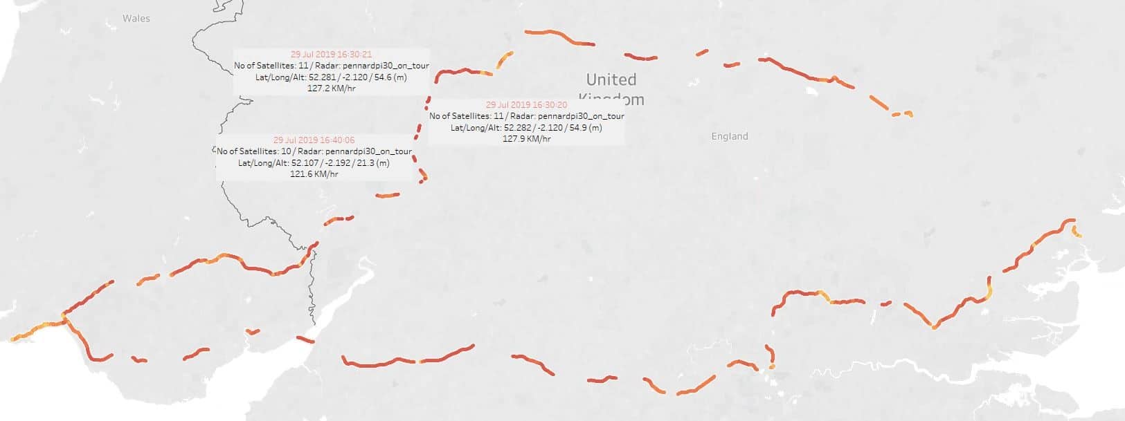
Prior to going into lockdown due to COVID-19, pennardpi401_on_tour would travel in my laptop bag. One of its first tours was to our London office (when we had one ;-)). For this I would drive to my local train station, walk from the carpark to catch a train for the 200 mile journey to London Paddington. I would then use the Underground to travel to Moorgate. Unfortunately, as it is not possible to pick up a GPS signal underground, this section of the journey would be devoid of data. I would then walk 10-15 minutes to the office in Wood Street. Several hours later, I would return home.
Other journeys included driving to meet one of our customers in Cambridge (UK) and another in Colchester, and further afield to Moscow, South Africa and elsewhere. However, just as I was not being able to pick up a GPS signal underground, when flying, I naturally had to switch off my mobile phone and RPI due to restrictions. Though you can but imagine the conversation I would have when I took the portable Raspberry Pi through airport security!
On each of these journeys I would periodically check in on the Vertica cluster to ensure the data was being ingested from Kafka. I could of course also use kafkacat to see the stream of messages in Kafka. I could check the Management Console to confirm the micro batches are loading and I could run simple SQL against the data in Vertica. So many options 🙂
But what I really liked to see was the data visualised in one of the many BI tools that work with Vertica. Although I have many options to choose from, I would often opt for Tableau – if for no other reason than I have a license for it. I would also use the likes of KNIME, and Jupyter Notebooks as open source alternatives – if for no other reason than to show I am not biased to one technology provider.
I have started to take the portable RPI with me when I go out for walks and on bike rides. Each time logging the data it captured, and being amazed at how accurate it was. Not only recording my location and direction of travel, but speed across the ground, altitude and number of satellites in view amongst other interesting metrics.
I could use the data to show how, not only would I lose GPS signal (for example being underground), but could identify blind spots for mobile phone signal. On the loss of mobile phone signal, one of the enhancements to my ETL application that I am considering is to retain the data that was unable to be live-streamed due to lack of signal, and to batch upload it when a signal can be re-established.
Another thought that I have had, and a challenge to those budding Data Scientists out there, is now I’ve got a series of journeys, for them to build some Machine Learning models to try and determine the mode of transport used. There are clearly some obvious characteristics of journeys done on foot, bike, car, train, boat etc.
More of that to come later.
The car does not need washing!
With the approval of SWMBO (She Who Must Be Obeyed – Bev, my wife and much better half!), I asked if I could put the portable RPI in her car as she went to our local supermarket to collect a pre-ordered grocery delivery.
Using Tableau, I tracked her as she drove from our house to an industrial estate on the outskirts of Swansea (remembering I had set the micro batch loading to be every 10 seconds, so could refresh my Tableau map whenever I wanted to). I noted that Bev pulled into the supermarket’s fuel station – where I thought she was going to refuel her car (the BMW X5 sport was a fuel-greedy beast, and thankfully she has recently changed it to an Audi Q5). But rather than stop at the fuel pump, she continued round to the exit, where I know there is a car wash/valet station.
At this point, I telephoned her and said “The car doesn’t need washing”. Needless to say, I will not be allowed to put the RPI in her car again!
Take nothing but memories. Leave nothing but footprints
After this rather long, but hopefully interesting story, I will come on to the final piece.
In an earlier post (COVID-19 Birdsong), I wrote about how quiet everything had gone in the countryside with COVID-19. Although we are far from being out of the woods with this pandemic, the UK started to take some tentative steps to easing the lockdown. Living in Wales, and under a devolved government (don’t get me started on that!), our restrictions are easing a little behind England – not that I am against that.
With the prospect of our public spaces starting to open up, including our award-winning beaches on the Gower Peninsula, I decided I needed to take advantage of this quiet time and make my mark.

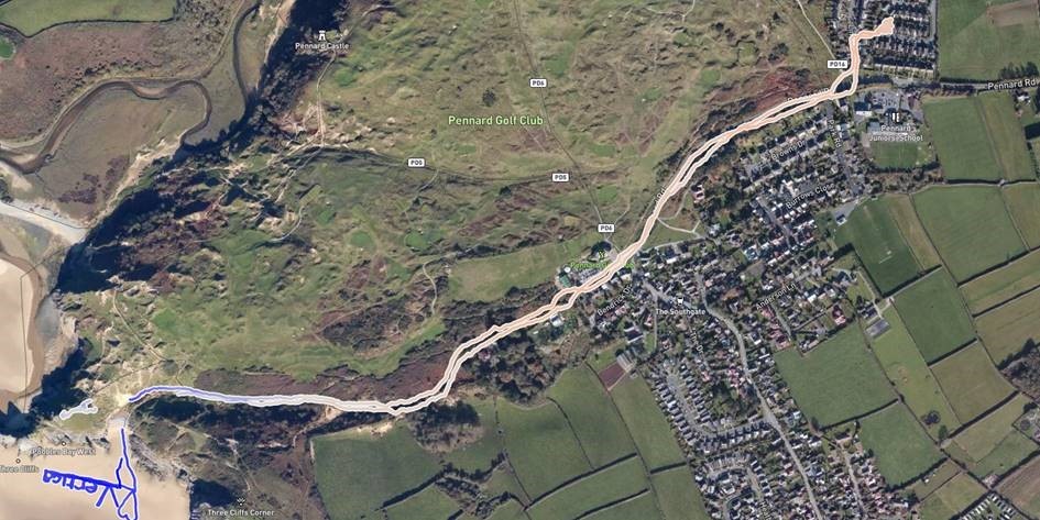
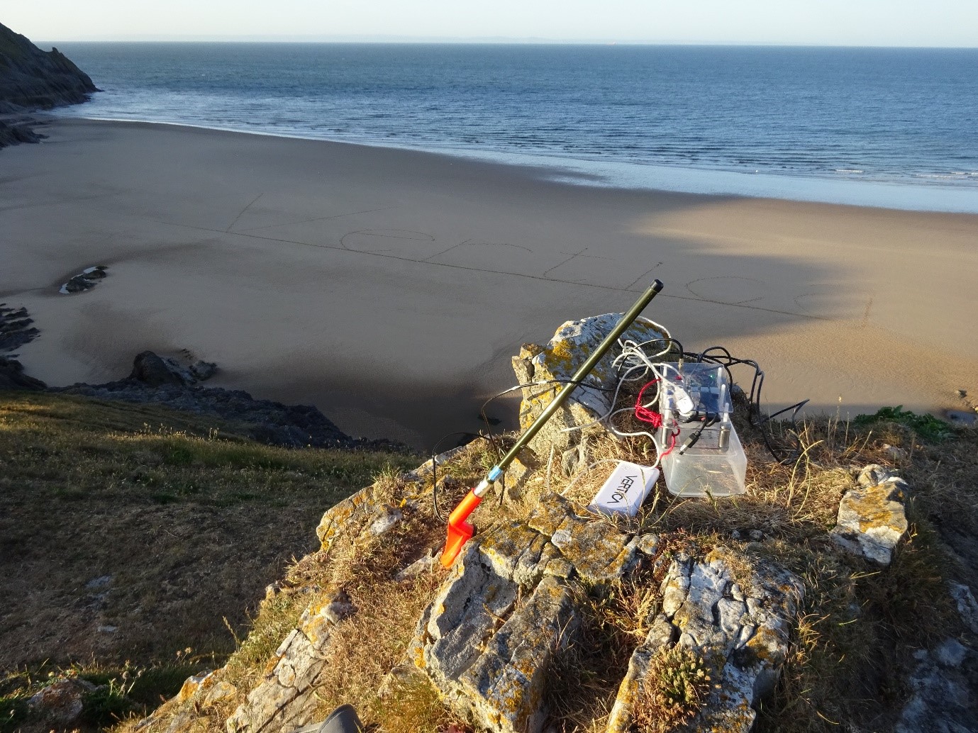
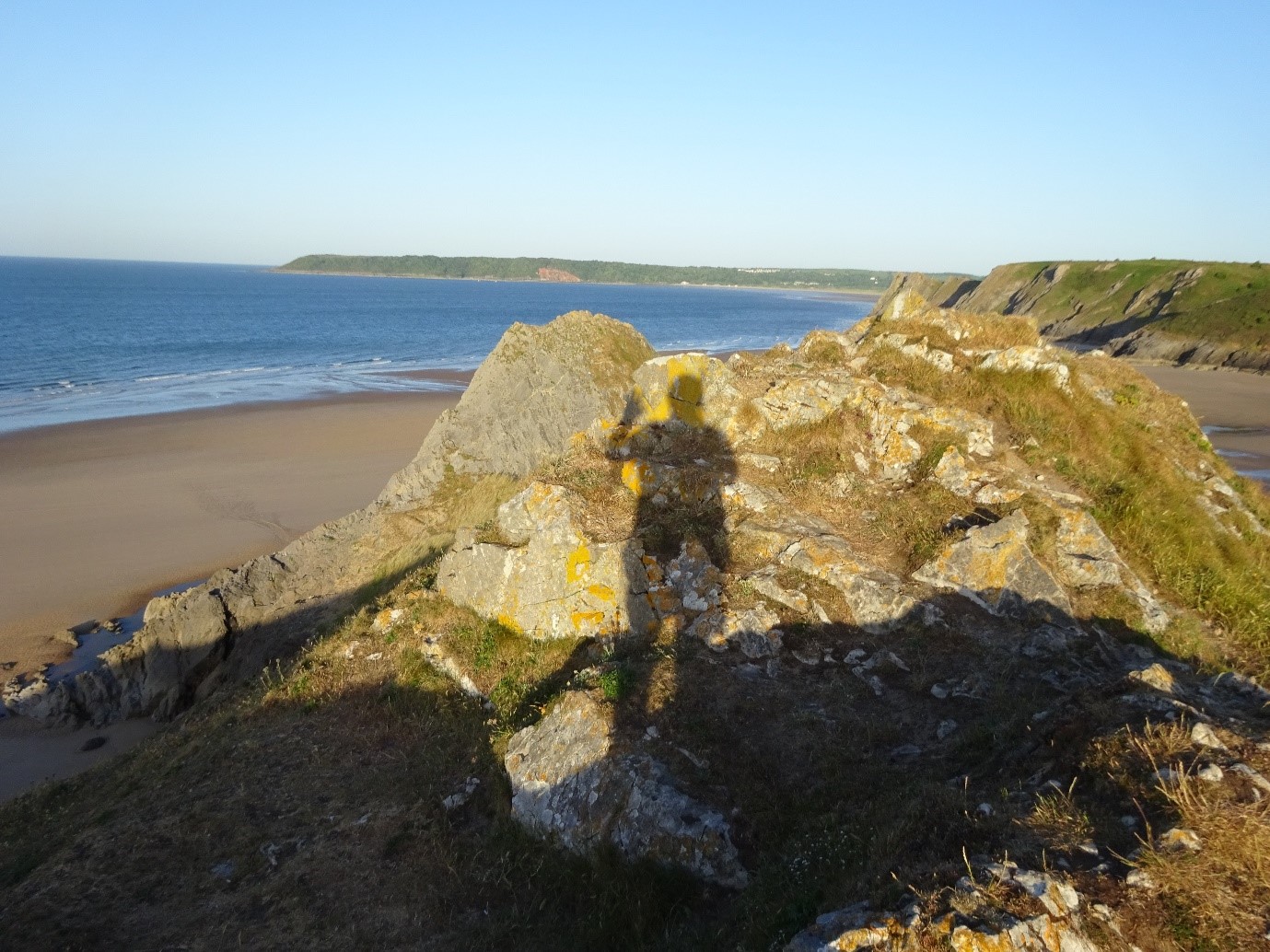
Setting off at approximately 05:00 AM, with my rucksack on my back (with pennardpi401 on board), I walked from my home, passing Pennard Golf Club. Thankfully, the golfers are still not allowed back to the links, and thus no need to duck the stray golf balls (see my Birdsong blog for more on this). A few minutes later I arrived at Three Cliffs and Pobbles Bays.
Just to be clear. The reason for the 05:00 AM start, was twofold. Firstly, at that time of the morning, I am unlikely to meet anyone else. Secondly, the tide is out – which for reference the Gower tides have the 2nd highest range in the world (13m / 43ft)!
With regard to my “take nothing but memories, leave nothing but footprints”, I have to own up, I did a bit more. Throughout my early-morning walk, I took 1,000s of GPS data point (and lots of photos). As for leaving nothing but footprints, I’m afraid those footprints turned into a 300m (1000 ft) piece of graffiti.
The following two images were generated from Tableau, pulling data out of the Vertica database. As with photos, this data can live inside Vertica forever. But unlike photos, I could now do analysis on this data. Such as calculating the total distance traveled, the average speed, the changes in altitude, how much faster was I going downhill than uphill.
But for this, I decided all I wanted to keep were the memories . . .
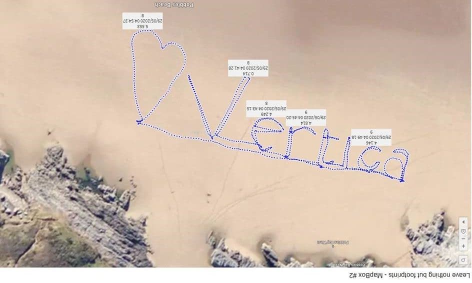
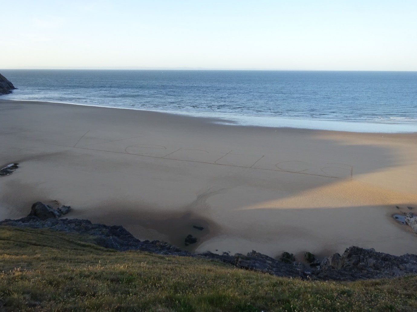
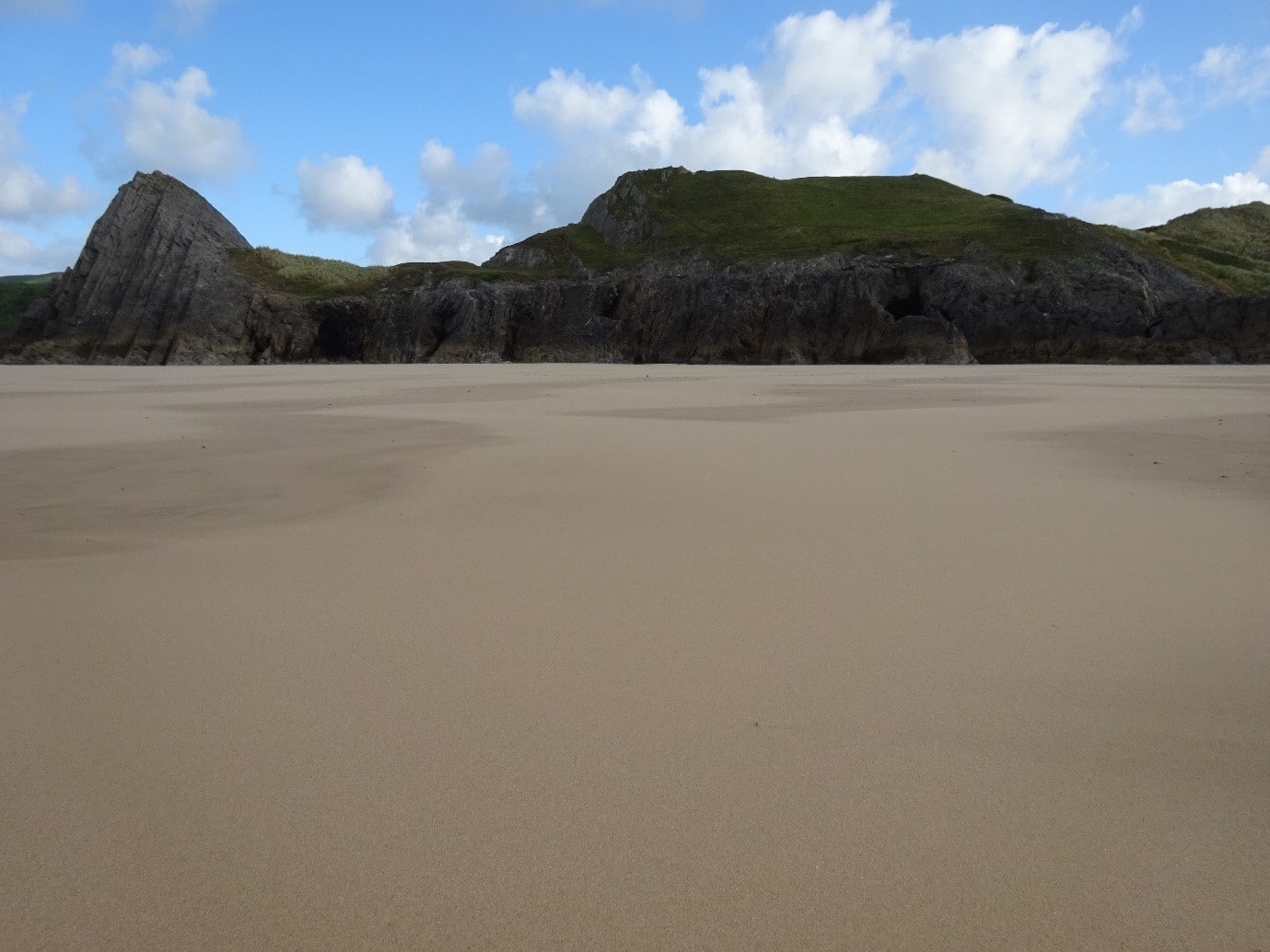
After completing the Vertica logo (which as I mentioned was ~300 m/1000 ft wide), I climbed up onto a cliff overlooking the beach and took some photos.
You may be able to see a couple of white specs near the waterline. The first directly above the “i” of Vertica, the second further over to the right. These are seagulls – so hopefully giving an idea of scale.
I was also a little disappointed that the heart I drew to the left of Vertica did not come out on the photo. Though thankfully I have the digital GPS data to prove I did it. Maybe the picture does sometimes “lie”.
After daubing graffiti all over Pobbles Bay, just like some of the more famous graffiti artists, I wasn’t going to take a picture of myself!
All swept clean
The good news, what I took (other than maybe some grains of sand between my toes), and what I left behind, had no negative impact on the environment. After my Vertica IoT data analytics beach excursion, the 13m tide that was on its way in, quickly washed away my footprints and graffiti back to a pristine, flawless clean beach.
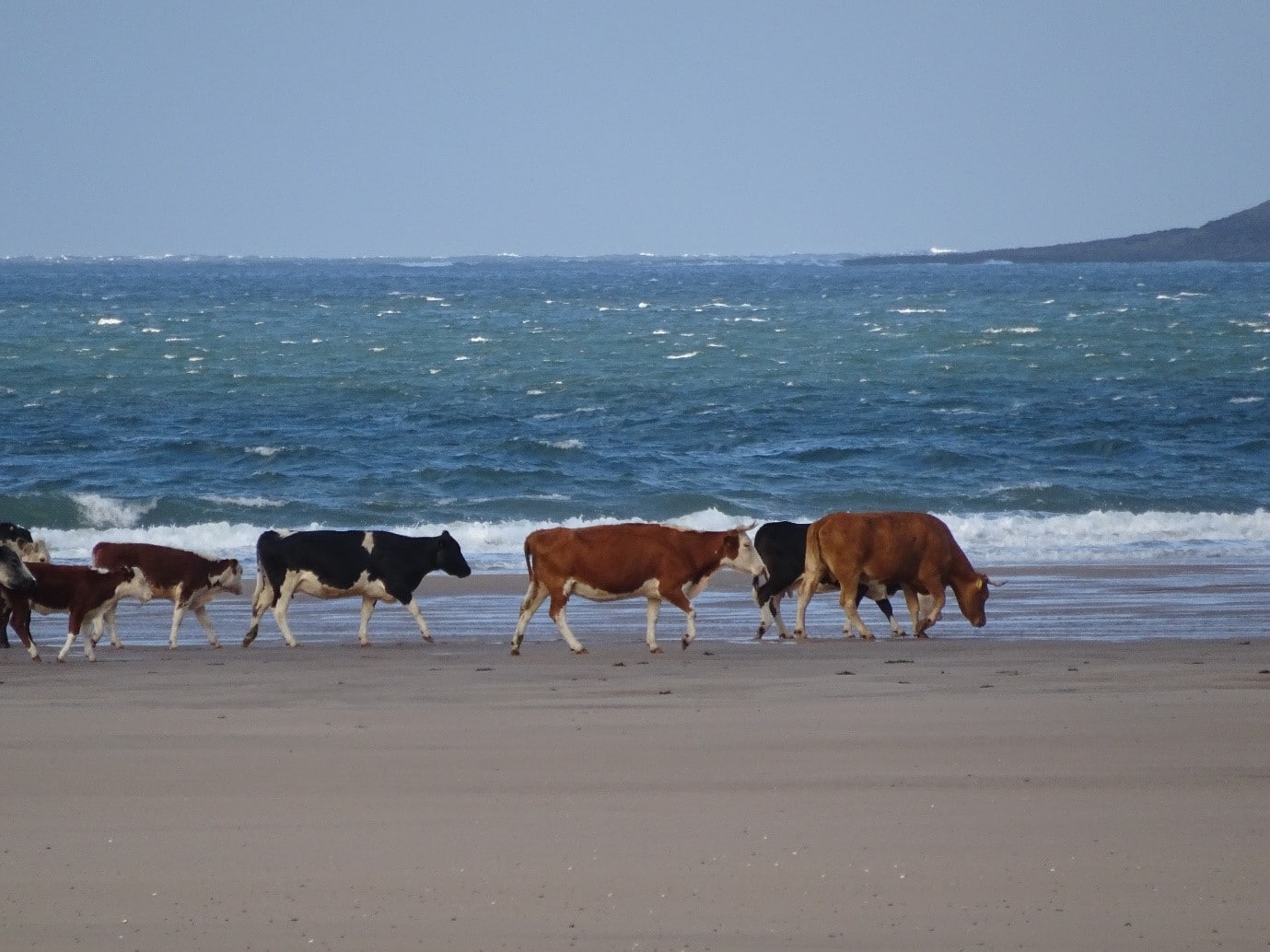
A few days later
Just a few days later, I went for another walk on the beach, only to find a herd of cattle taking an early morning bath. Just wondered if they were going to leave “something” behind?
About the Author
Mark Whalley
Manager, Vertica Education
From the early 1980s, Mark worked with Michael Stonebraker's Ingres RDBMS and then a number of column-store big data analytics technologies.
In 2016, he joined HPE Big Data Platform as a Systems Engineer specialising in Stonebraker’s Vertica.
In September 2017 he followed Vertica as it merged into Micro Focus – one of the world’s largest pure-play software companies.
He is passionate about technology and frequently delivers talks at the London, Cambridge and Munich Big Data & Machine Learning Meetups (of which he is the founder with its 4K+ members), the British Computer Society – Advanced Programming Specialist Group, Vertica Forums, the Institute for Analytics and Data Science at the University of Essex et al.
He is a technical blogger and author.