


SQL query results Graphic Options
There are many ways to present query results in graphics but no references were found about how to do it only with SQL natively. For example: – Tableau Software generates interactive data visualization focused on business intelligence. – MicroStrategy provides BI, mobile software, and cloud-based services, to analyze internal and external data. – Highcharts is being used by over 80% of the largest companies in the world. There are 2.6 Million code references to Highcharts on GitHub. – R provides strong graphic capabilities. – DbVisualizer and similar BI/SQL front-end tools. – VPython and Jupyter notebook makes it easy to create navigable real-time 3D animations. – Vander produces a live-graph on your terminal from integer output. – Flame Graphs provides visualization of profiled software. – Plotly reads data from a MySQL database and graphs it in Python.What is VSQL?
VSQL is Vertica’s character-based front-end utility used to enter SQL statements and display the results. It also provides a number of meta-commands and various shell-like features that make it easier to write scripts. The VSQL client utility is available as part of the Vertica server rpm installation or as a client Driver package downloaded from https://my.vertica.com/download. In addition to SQL commands, VSQL supports Meta Commands, processed by vsql to make vsql more useful for scripting. Any VSQL argument in single quotes is subject to C-like substitutions for \n (new line), \t (tab), \digits, \0digits, and \0xdigits (the character with the given decimal, octal, or hexadecimal code). One of the common meta-commands used here is the \set command to set an internal variables with values. When multiple values are specified, they are concatenated. An unqualified \set command lists all internal variables.How to run this demo
VSQL can run as a client locally on Windows and connect to the Vertica database remotely, or run directly on a Vertica Linux host as this demo does. A direct connection effectively ensures consistent performance with less chance of delays and dropped connections, and reduces data transfer costs associated with cloud deployments. The SQL code in this demo is intended to run in Vertica VSQL Bash environment, but Bash does not define colors. Everything depends on your terminal emulator (vt100, vt200, xterm, gnome-terminal etc.) capabilities to “understand colors”. Note that this demo uses a mixture of “tput” commands and escape sequence to present graphics. However, there is a risk that another terminal emulator might use an entirely different set of characters to represent those colors. This is why we should first test our target environment and always prefer “tput” use in a production environment. When you run tput xyz, tput checks the terminal’s escape codes for the color xyz and outputs the relevant escape code. “tput” produces character sequences interpreted by the terminal emulators as having a special meaning. To download the SQL demo script: Right-click [HERE] and select Save Link As: vdraw.sql. This script includes data sample, data generate commands, and COPY commands, you can use to try the SQL code on real data, in a test environment. Usage:vsql -qf vdraw.sql
VT Terminal Escape Sequences
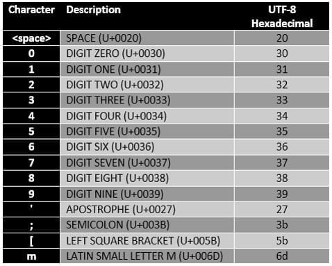
VT terminal emulators support colors and graphic symbols through a system of escape sequences. Several terminal specifications are based on the ANSI color standard, including VT100. Using the following conversion tables, set multiple VT terminal display attribute modes with: [{attribute1};…;{attributeN}m. Standard VTx00 Decimal colors example: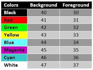 UTF-8 encoding and Unicode characters example:
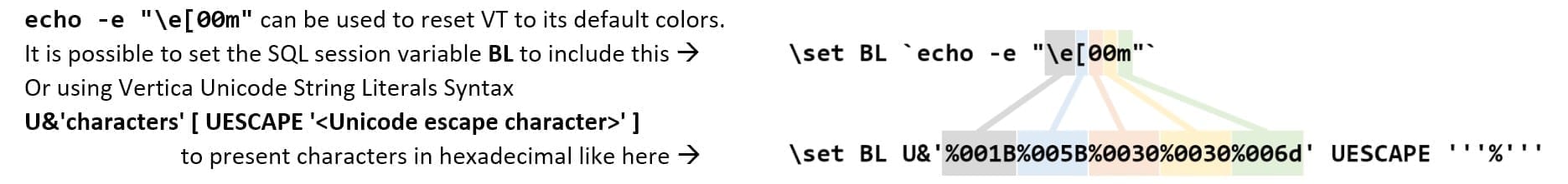
Vertica Unicode String Literals Syntax example
Vertica table with ANSI color-codes example
To make it more usable by any session, we can create a Vertica permanent table with ANSI color codes, special characters, and cursor control codes:CREATE TABLE colors(
cid int, bold varchar, unbold varchar, mark varchar, white varchar,
red varchar,b_dark_blue varchar, b_light_blue varchar, b_d_red varchar,
b_d_green varchar, b_brown varchar, b_purple varchar, b_turquoise varchar,
b_l_gray varchar, b_d_gray varchar, b_l_red varchar, b_l_green varchar,
b_yellow varchar, b_pink varchar, b_vl_blue varchar, green varchar,
green_font varchar, red_font varchar, yellow_font varchar, black varchar,
begin_underline varchar, end_underline varchar)
UNSEGMENTED ALL NODES KSAFE 0;
INSERT INTO colors (cid, bold, unbold, mark,white,red,b_dark_blue,b_light_blue,
b_d_red, b_d_green, b_brown,b_purple, b_turquoise, b_l_gray,
b_d_gray, b_l_red, b_l_green, b_yellow, b_pink, b_vl_blue, green,
green_font,red_font,yellow_font,black,begin_underline,end_underline)
values (1, :BOLD, :UNBOLD, :MARK, :WH, :RE, :B_D_BLUE, :B_L_BLUE, :B_D_RED,
:B_D_GREEN, :B_BROWN,:B_PURPLE,:B_TURQUOISE, :B_L_GRAY, :B_D_GRAY,
:B_L_RED, :B_L_GREEN, :B_YELLOW, :B_PINK, :B_VL_BLUE,
:GR, :GRonBL, :REonBL, :YLonBL, :BL, :BU, :EU);
Later on, using the following result set, we can present colors using the stored colors in the table as shown below:
SELECT id,INSERT(INSERT(REPEAT('_', id) || REPEAT(' ', 100-id),id+1,0,black),1,0,white)
as :TITLE ,value
FROM            resultset01, colors
WHERE           colors.cid=1
ORDER BY        resultset01.id DESC;
which displays the following graphic:
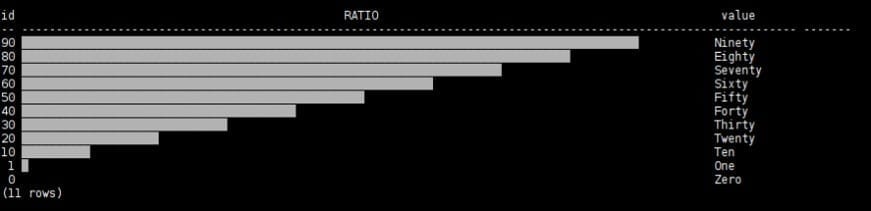
The following few graphs use this result set:
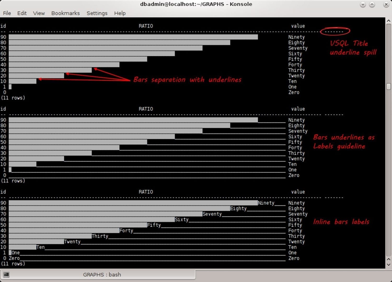
Most of the graph examples use background colors to present text labels inside, or in combination with, the graph bars. Underline mode is used to emphasize each bar boundary as a line separation between the bars.
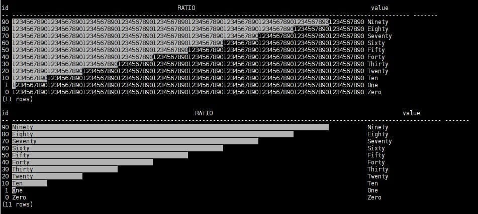
Vertica VSQL calculates each result set column and titles width. Hence, graphs with unprintable characters and default VSQL tabling alignment and delimiters cause titles and its underline to spill (See below).
That is why, later in this document, we will turn off VSQL titles using meta-commands to toggle output format: \a (alignment), \t (tuples only). In some graphs, we will manage the titles ourselves with the same SQL query code.
result_version barid id normalised_id  value
-------------- ----- -- ------------- -------
             1        0               Zero
             1        1               One
             1       10               Ten
             1       20               Twenty
             1       30               Thirty
             1       40               Forty
             1       50               Fifty
             1       60               Sixty
             1       70               Seventy
             1       80               Eighty
             1       90               Ninety
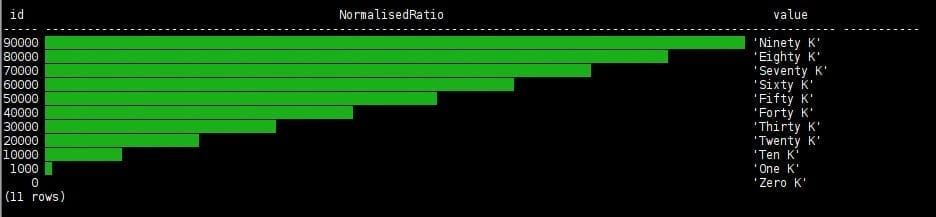
Compression Ratio
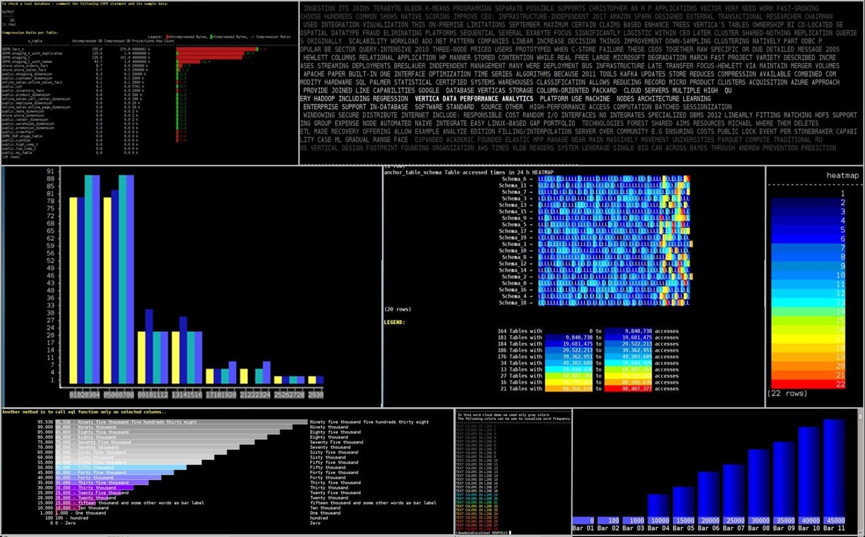
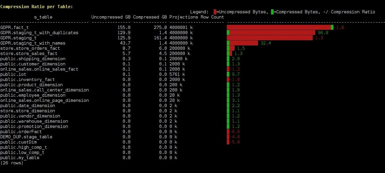
By grouping data together on disk by column, Vertica creates the perfect scenario for data compression because many similar values can be compressed very aggressively. In addition, Vertica DBD with the Vertica built-in function, ANALYZE_CORRELATIONS, analyzes the database tables for columns that are strongly correlated. It is intended to produce an optimal design to increase the ratio between the input, uncompressed raw data, size, and its ROSs compressed size. Vertica features a library of many compression algorithms, which it applies automatically based on data type. Typically, the data in Vertica occupies much less disk space than the data loaded into it. This not only lowers storage costs, but also speeds up querying by further reducing disk I/O. The next graph example shows your database compression ratio per table. The calculation based on USER_AUDITS audits is generated by calling the AUDIT function. Hence, to obtain the latest audits we audit those tables fast, like so:SELECT AUDIT('','TABLE',5,99);
This audits the entire database with Table granularity, error‑tolerance=5, confidence‑level=99%. The provided demo script loads sample data to draw the graph below. To check a real database, comment its COPY statement and its sample data.
First, create a table on the initiator node only, to hold the query results locally. A temporary table does not overburden the Vertica Catalog and with “KSAFE 0” it will not create buddy projections:
CREATE LOCAL TEMPORARY TABLE resultset02
(
result_version                      int,
s_table                             varchar(80),
compressed_bytes                    int,
normalised_compressed_bytes         int,
uncompressed_Bytes                  int,
normalised_uncompressed_Bytes       int,
projections_row_count               int,
compression_ratio                   numeric,
normalised_compression_ratio        numeric
)
ON COMMIT PRESERVE ROWS
KSAFE 0;
Use the following code to calculate and save the compression ratio per table:
INSERT INTO resultset02(result_version,
s_table,
compressed_bytes,
uncompressed_bytes,
projections_row_count,
compression_ratio)
WITH
MAXUA AS
(SELECT audited_schema_name || '.' || audited_object_name AS S_TABLE,
object_type,
MAX(audit_end_timestamp) AS MAXAUDIT
FROM v_catalog.user_audits
WHERE object_type = 'TABLE'
GROUP BY 1,2),
PS AS
(SELECT anchor_table_schema || '.' || anchor_table_name AS S_TABLE,
SUM(used_bytes) AS compressed_bytes,
sum(row_count)  AS projections_row_count
FROM   v_monitor.projection_storage
GROUP BY 1)
SELECT 1 AS result_version,
UA.audited_schema_name || '.' || UA.audited_object_name          AS s_table,
PS.compressed_bytes::NUMERIC(20,0)                               AS compressed_bytes,
UA.size_bytes::NUMERIC(20,0)                                     AS uncompressed_bytes,
PS.projections_row_count                                         AS projections_row_count,
(UA.size_bytes / NULLIFZERO(PS.compressed_bytes))::NUMERIC(10,1) AS compression_ratio
FROM v_catalog.user_audits UA, MAXUA, PS
WHERE UA.object_type = 'TABLE'
AND UA.audited_schema_name || '.' || UA.audited_object_name = MAXUA.S_TABLE
AND PS.S_TABLE = MAXUA.S_TABLE
AND UA.audit_end_timestamp = MAXUA.MAXAUDIT
ORDER BY 2 desc;
The red color represents uncompressed /bytes and green colors represent compressed Bytes.
Note that when the compressed size is larger than the original uncompressed raw data that the compression ratio number is negative in red color. In addition, when a negative compression ratio is presented, the bar starts as a red bar and not green:
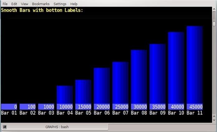
Vertical Bars
Vertical bars presented with smooth background colors and top or bottom labels like shown in several options in the provided script. In contrast to horizon bars, the drawback of vertical bars is that the amount of the bars number is limited and planned in advance. Here is the SQL code example used to produce the vertical bar chart below:\f ' '
\a
\t
\pset border 0
WITH BARST AS
(SELECT SUM(CASE WHEN barid=1 THEN normalised_id ELSE 0 END) AS barid_1, SUM(CASE WHEN barid=1 THEN id ELSE 0 END) AS id_1,
SUM(CASE WHEN barid=2 THEN normalised_id ELSE 0 END) AS barid_2, SUM(CASE WHEN barid=2 THEN id ELSE 0 END) AS id_2,
SUM(CASE WHEN barid=3 THEN normalised_id ELSE 0 END) AS barid_3, SUM(CASE WHEN barid=3 THEN id ELSE 0 END) AS id_3,
SUM(CASE WHEN barid=4 THEN normalised_id ELSE 0 END) AS barid_4, SUM(CASE WHEN barid=4 THEN id ELSE 0 END) AS id_4,
SUM(CASE WHEN barid=5 THEN normalised_id ELSE 0 END) AS barid_5, SUM(CASE WHEN barid=5 THEN id ELSE 0 END) AS id_5,
SUM(CASE WHEN barid=6 THEN normalised_id ELSE 0 END) AS barid_6, SUM(CASE WHEN barid=6 THEN id ELSE 0 END) AS id_6,
SUM(CASE WHEN barid=7 THEN normalised_id ELSE 0 END) AS barid_7, SUM(CASE WHEN barid=7 THEN id ELSE 0 END) AS id_7,
SUM(CASE WHEN barid=8 THEN normalised_id ELSE 0 END) AS barid_8, SUM(CASE WHEN barid=8 THEN id ELSE 0 END) AS id_8,
SUM(CASE WHEN barid=9 THEN normalised_id ELSE 0 END) AS barid_9, SUM(CASE WHEN barid=9 THEN id ELSE 0 END) AS id_9,
SUM(CASE WHEN barid=10 THEN normalised_id ELSE 0 END) AS barid_10, SUM(CASE WHEN barid=10 THEN id ELSE 0 END) AS id_10,
SUM(CASE WHEN barid=11 THEN normalised_id ELSE 0 END) AS barid_11, SUM(CASE WHEN barid=11 THEN id ELSE 0 END) AS id_11
FROM resultset01),
MYROWS as (select row_number() over() -3 as rid from
( select 1 from ( select now() as se union all select now() + :GRAPH_HIGHT as se) a
timeseries ts as '1 day' over (order by se)) b)
select
CASE WHEN rid = -1 THEN CHR(27) || b_light_blue || to_char(id_1,'99999') || black WHEN rid = -2 THEN 'Bar 01' WHEN barid_1 > rid THEN :BAR5 ELSE ' ' END AS id_1,
CASE WHEN rid = -1 THEN CHR(27) || b_light_blue || to_char(id_2,'99999') || black WHEN rid = -2 THEN 'Bar 02' WHEN barid_2 > rid THEN :BAR5 ELSE ' ' END AS id_2,
CASE WHEN rid = -1 THEN CHR(27) || b_light_blue || to_char(id_3,'99999') || black WHEN rid = -2 THEN 'Bar 03' WHEN barid_3 > rid THEN :BAR5 ELSE ' ' END AS id_3,
CASE WHEN rid = -1 THEN CHR(27) || b_light_blue || to_char(id_4,'99999') || black WHEN rid = -2 THEN 'Bar 04' WHEN barid_4 > rid THEN :BAR5 ELSE ' ' END AS id_4,
CASE WHEN rid = -1 THEN CHR(27) || b_light_blue || to_char(id_5,'99999') || black WHEN rid = -2 THEN 'Bar 05' WHEN barid_5 > rid THEN :BAR5 ELSE ' ' END AS id_5,
CASE WHEN rid = -1 THEN CHR(27) || b_light_blue || to_char(id_6,'99999') || black WHEN rid = -2 THEN 'Bar 06' WHEN barid_6 > rid THEN :BAR5 ELSE ' ' END AS id_6,
CASE WHEN rid = -1 THEN CHR(27) || b_light_blue || to_char(id_7,'99999') || black WHEN rid = -2 THEN 'Bar 07' WHEN barid_7 > rid THEN :BAR5 ELSE ' ' END AS id_7,
CASE WHEN rid = -1 THEN CHR(27) || b_light_blue || to_char(id_8,'99999') || black WHEN rid = -2 THEN 'Bar 08' WHEN barid_8 > rid THEN :BAR5 ELSE ' ' END AS id_8,
CASE WHEN rid = -1 THEN CHR(27) || b_light_blue || to_char(id_9,'99999') || black WHEN rid = -2 THEN 'Bar 09' WHEN barid_9 > rid THEN :BAR5 ELSE ' ' END AS id_9,
CASE WHEN rid = -1 THEN CHR(27) || b_light_blue || to_char(id_10,'99999') || black WHEN rid = -2 THEN 'Bar 10' WHEN barid_10 > rid THEN :BAR5 ELSE ' ' END AS id_10,
CASE WHEN rid = -1 THEN CHR(27) || b_light_blue || to_char(id_11,'99999') || black WHEN rid = -2 THEN 'Bar 11' WHEN barid_11 > rid THEN :BAR5 ELSE ' ' END AS id_11
FROM BARST, MYROWS, colors
WHERE colors.cid=1
ORDER BY MYROWS.rid DESC;
The SQL code above will produce this graph:
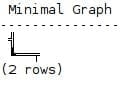
Tailor-made Bar Charts – ROS containers count
The Y-axis (╣) and X-axis ( ═╤ ) defined in the following example produced the minimal graph below:\set Y_AXIS U&'%2563' UESCAPE '''%''' \set X_AXIS0 U&'%2517' UESCAPE '''%''' \set X_AXIS1 U&'%2550' UESCAPE '''%''' \set X_AXIS2 U&'%2550%2564' UESCAPE '''%''' SELECT :Y_AXIS AS 'Minimal Graph' UNION ALL SELECT :X_AXIS0 || :X_AXIS1 || :X_AXIS2;
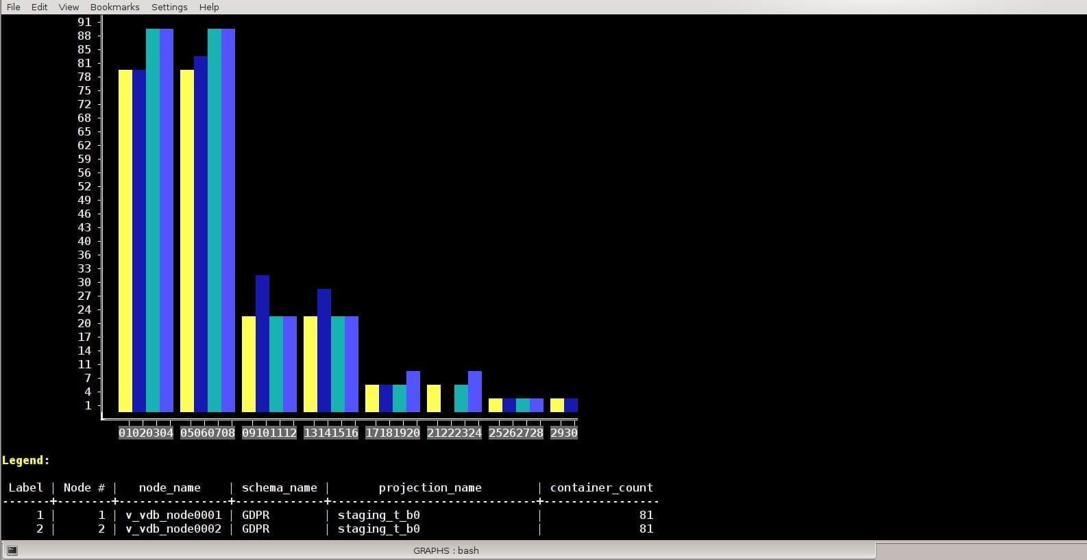
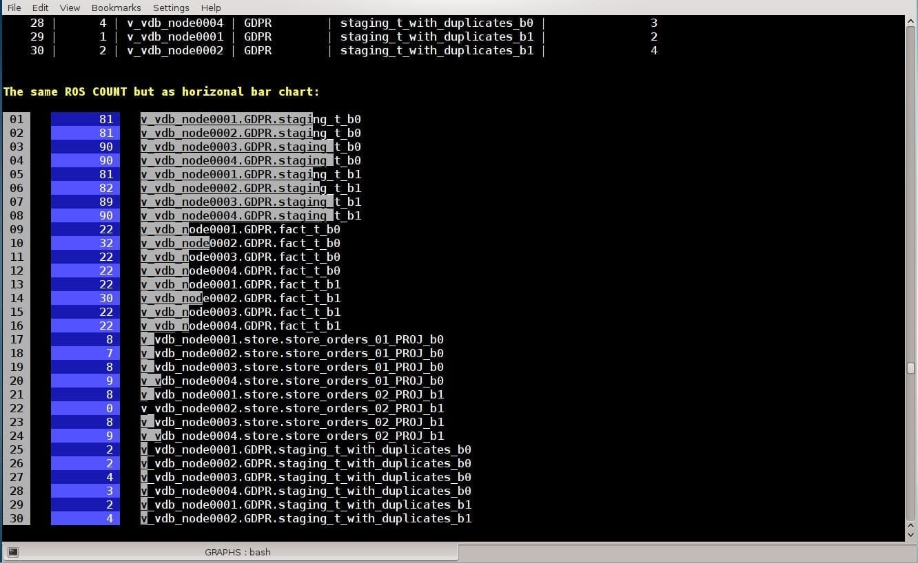
 The following tailor made vertical bar chart changes the bars to order and groups the bars to compare the ROS containers count
between the same projections on different nodes.
The sample data used demonstrates unusual phenomena with high differences in the projection sizes to make the graph interesting. One can delete the sample data and try the code in a QA environment to examine its own projection sizes, likely to verify that all projections are evenly spread between the nodes.
Legend:
The following tailor made vertical bar chart changes the bars to order and groups the bars to compare the ROS containers count
between the same projections on different nodes.
The sample data used demonstrates unusual phenomena with high differences in the projection sizes to make the graph interesting. One can delete the sample data and try the code in a QA environment to examine its own projection sizes, likely to verify that all projections are evenly spread between the nodes.
Legend:
 Label | Node # |   node_name    | schema_name |       projection_name        | container_count
-------+--------+----------------+-------------+------------------------------+-----------------
     1 |      1 | v_vdb_node0001 | GDPR        | staging_t_b0                 |              81
     2 |      2 | v_vdb_node0002 | GDPR        | staging_t_b0                 |              81
     3 |      3 | v_vdb_node0003 | GDPR        | staging_t_b0                 |              90
     4 |      4 | v_vdb_node0004 | GDPR        | staging_t_b0                 |              90
     5 |      1 | v_vdb_node0001 | GDPR        | staging_t_b1                 |              81
     6 |      2 | v_vdb_node0002 | GDPR        | staging_t_b1                 |              82
     7 |      3 | v_vdb_node0003 | GDPR        | staging_t_b1                 |              89
     8 |      4 | v_vdb_node0004 | GDPR        | staging_t_b1                 |              90
     9 |      1 | v_vdb_node0001 | GDPR        | fact_t_b0                    |              22
    10 |      2 | v_vdb_node0002 | GDPR        | fact_t_b0                    |              32
    11 |      3 | v_vdb_node0003 | GDPR        | fact_t_b0                    |              22
    12 |      4 | v_vdb_node0004 | GDPR        | fact_t_b0                    |              22
    13 |      1 | v_vdb_node0001 | GDPR        | fact_t_b1                    |              22
    14 |      2 | v_vdb_node0002 | GDPR        | fact_t_b1                    |              30
    15 |      3 | v_vdb_node0003 | GDPR        | fact_t_b1                    |              22
    16 |      4 | v_vdb_node0004 | GDPR        | fact_t_b1                    |              22
    17 |      1 | v_vdb_node0001 | store       | store_orders_01_PROJ_b0      |               8
    18 |      2 | v_vdb_node0002 | store       | store_orders_01_PROJ_b0      |               7
    19 |      3 | v_vdb_node0003 | store       | store_orders_01_PROJ_b0      |               8
    20 |      4 | v_vdb_node0004 | store       | store_orders_01_PROJ_b0      |               9
    21 |      1 | v_vdb_node0001 | store       | store_orders_02_PROJ_b1      |               8
    22 |      2 | v_vdb_node0002 | store       | store_orders_02_PROJ_b1      |               0
    23 |      3 | v_vdb_node0003 | store       | store_orders_02_PROJ_b1      |               8
    24 |      4 | v_vdb_node0004 | store       | store_orders_02_PROJ_b1      |               9
    25 |      1 | v_vdb_node0001 | GDPR        | staging_t_with_duplicates_b0 |               2
    26 |      2 | v_vdb_node0002 | GDPR        | staging_t_with_duplicates_b0 |               2
    27 |      3 | v_vdb_node0003 | GDPR        | staging_t_with_duplicates_b0 |               4
    28 |      4 | v_vdb_node0004 | GDPR        | staging_t_with_duplicates_b0 |               3
    29 |      1 | v_vdb_node0001 | GDPR        | staging_t_with_duplicates_b1 |               2
    30 |      2 | v_vdb_node0002 | GDPR        | staging_t_with_duplicates_b1 |               4
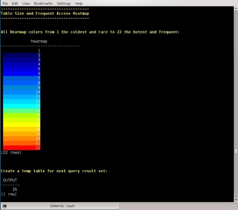
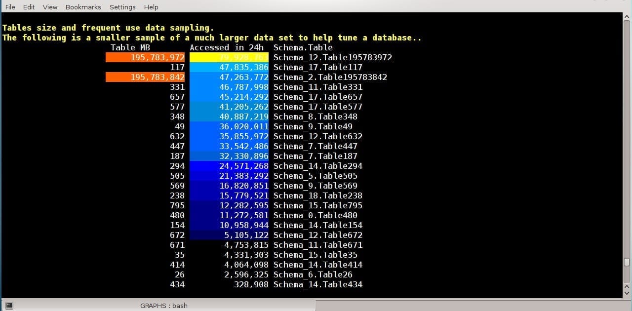
Vertica Tables Size and Frequent Access Heatmap
All Heatmap colors from one (the coldest and rare) to 22 (the hottest and frequent) presented via the function heatmap as follows:CREATE OR REPLACE FUNCTION heatmap (heat INT, value INT)
RETURN VARCHAR
AS BEGIN
RETURN CHR(27) || '[48;5;' ||
CASE
WHEN heat < 1 THEN '16'
WHEN MOD(heat,22) = 0 THEN '196'
WHEN MOD(heat,21) = 0 THEN '202'
WHEN MOD(heat,20) = 0 THEN '208'
WHEN MOD(heat,19) = 0 THEN '214'
WHEN MOD(heat,18) = 0 THEN '220'
WHEN MOD(heat,17) = 0 THEN '226'
WHEN MOD(heat,16) = 0 THEN '190'
WHEN MOD(heat,15) = 0 THEN '154'
WHEN MOD(heat,14) = 0 THEN '84'
WHEN MOD(heat,13) = 0 THEN '51'
WHEN MOD(heat,12) = 0 THEN '45'
WHEN MOD(heat,11) = 0 THEN '39'
WHEN MOD(heat,10) = 0 THEN '33'
WHEN MOD(heat,9) = 0 THEN '32'
WHEN MOD(heat,8) = 0 THEN '27'
WHEN MOD(heat,7) = 0 THEN '26'
WHEN MOD(heat,6) = 0 THEN '21'
WHEN MOD(heat,5) = 0 THEN '20'
WHEN MOD(heat,4) = 0 THEN '19'
WHEN MOD(heat,3) = 0 THEN '18'
WHEN MOD(heat,2) = 0 THEN '17'
ELSE '16'
END ||
'm' || TO_CHAR(value,'999,999,999,999') || CHR(27) || :DEFAULT_C ;
END ;
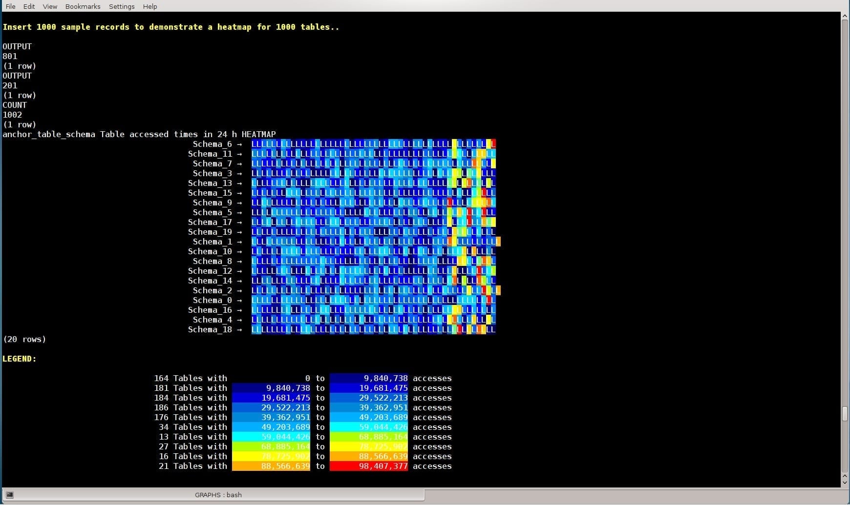
INSERT INTO table_size_and_freq_use (result_version, anchor_table_schema, anchor_table_name, MB, max_accessed_in_24_hours)
WITH
frequent AS
(SELECT table_schema, table_name, time_slice(time, 24, 'HOUR') AS time_window, COUNT(*) AS accessed
FROM dc_projections_used
GROUP BY 1,2,3),
maxi  AS
(SELECT table_schema, table_name, MAX(accessed) AS max_accessed_in_24_hours
FROM frequent
GROUP BY 1,2
ORDER BY 3 DESC),
tblsize AS
(SELECT
anchor_table_schema,
anchor_table_name,
(SUM(used_bytes)/1024/1024)::numeric(7,3) as MB
FROM projection_storage
GROUP BY 1,2
ORDER BY 1 desc)
SELECT 1,
tblsize.anchor_table_schema,
tblsize.anchor_table_name,
tblsize.MB,
maxi.max_accessed_in_24_hours
FROM tblsize, maxi
WHERE maxi.table_schema = tblsize.anchor_table_schema AND
maxi.table_name = tblsize.anchor_table_name
ORDER BY 3 DESC;
Vertica Tables’ Size and Frequent Access heatmap:
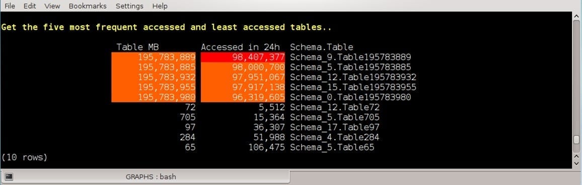
WITH maxi AS
(SELECT MAX(max_accessed_in_24_hours)::INT AS top_max
FROM table_size_and_freq_use
WHERE result_version =
(SELECT MAX(result_version)
FROM table_size_and_freq_use))
(SELECT REPEAT(' ',20) AS '    ',
heatmap(normelize(22,
(SELECT max(MB)::INT
FROM table_size_and_freq_use),MB::INT),MB::INT) AS '                 Table MB      ',
heatmap(normelize(22,top_max::INT,max_accessed_in_24_hours::INT),
max_accessed_in_24_hours::INT) AS ' Accessed in 24h',
anchor_table_schema || '.' || anchor_table_name AS ' Schema.Table'
FROM table_size_and_freq_use, maxi
WHERE result_version =
(SELECT MAX(result_version)
FROM table_size_and_freq_use)
ORDER BY table_size_and_freq_use.max_accessed_in_24_hours DESC
LIMIT 5)
UNION ALL
(SELECT REPEAT(' ',20) AS '    ',
heatmap(normelize(22,
(SELECT max(MB)::INT
FROM table_size_and_freq_use),MB::INT),MB::INT) AS '                 Table MB      ',
heatmap(normelize(22,top_max::INT,max_accessed_in_24_hours::INT),max_accessed_in_24_hours::INT) AS ' Accessed in 24h',
anchor_table_schema || '.' || anchor_table_name AS ' Schema.Table'
FROM table_size_and_freq_use, maxi
WHERE result_version =
(SELECT MAX(result_version)
FROM table_size_and_freq_use)
ORDER BY table_size_and_freq_use.max_accessed_in_24_hours ASC
LIMIT 5) ;
WITH
maxi AS (SELECT MAX(max_accessed_in_24_hours)::INT AS top_max
FROM table_size_and_freq_use
WHERE result_version = (SELECT MAX(result_version) FROM table_size_and_freq_use))
SELECT
REPEAT(' ',20) AS ' ', heatmap(normelize(22,(SELECT max(MB)::INT FROM table_size_and_freq_use),MB::INT),MB::INT)
AS '                    Table MB      ',   -- Table size in MB
heatmap(normelize(22,top_max::INT,max_accessed_in_24_hours::INT),max_accessed_in_24_hours::INT)
AS ' Accessed in 24h',
anchor_table_schema || '.' || anchor_table_name AS ' Schema.Table'
FROM maxi, table_size_and_freq_use TABLESAMPLE(3)
WHERE result_version = (SELECT MAX(result_version) FROM table_size_and_freq_use)
ORDER BY table_size_and_freq_use.max_accessed_in_24_hours DESC;
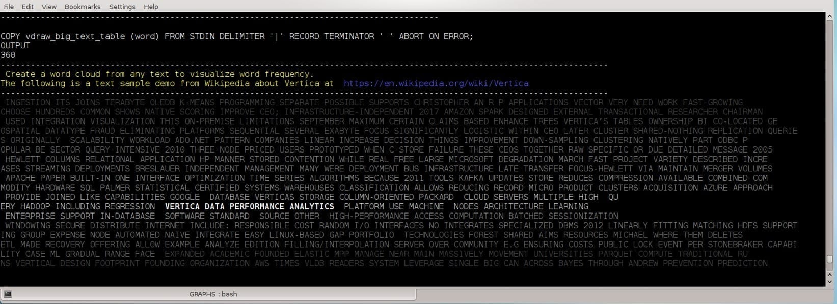
Word Cloud
The following example prints a wordcloud for a text of “Vertica” definition found in Wikipedia. First, we load the text to a table of words, clean conjunctions, SELECT GROUP BY the words, and then use the function line_color with one INT parameter: color_id. To handle big amounts, we prefer to color a group of words, not each ,word to reduce the amount of unprintable characters each word can be wrapped with. This example uses gray shades although the function can produce 28 colors for higher words with frequent presentations: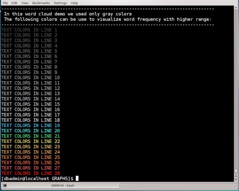
INSERT INTO resultset03(word, wcount, word_id, print_order)
WITH
words AS (SELECT UPPER(TRIM(BOTH ' `~.,-[      ]()’' FROM word)) AS word, COUNT(1) AS wcount
FROM vdraw_big_text_table
WHERE UPPER(TRIM(BOTH ' `~.,-[      ]()’' FROM word)) not in ('AND','THE','OF','TO','IN','A','WITH','FOR','ON','AS','WAS','BY','SUCH','AT',
'IS','WHICH','ARE','ALSO')
GROUP BY 1
ORDER BY 2 DESC),
tagid AS (SELECT word, wcount, row_number() over() as word_id
FROM words
ORDER BY wcount DESC),
words_count AS (SELECT count(1) AS maxid FROM tagid)
SELECT word, wcount, word_id,
CASE
WHEN word_id between CEIL(maxid * 0.9)  and maxid THEN 1
WHEN word_id between CEIL(maxid * 0.7)  and CEIL(maxid * 0.8)  THEN 2
WHEN word_id between CEIL(maxid * 0.5)  and CEIL(maxid * 0.6)  THEN 3
WHEN word_id between CEIL(maxid * 0.3)  and CEIL(maxid * 0.4)  THEN 4
WHEN word_id between CEIL(maxid * 0.1)  and CEIL(maxid * 0.2)  THEN 5
WHEN word_id between CEIL(maxid * 0.08) and CEIL(maxid * 0.09) THEN 6
WHEN word_id between CEIL(maxid * 0.06) and CEIL(maxid * 0.07) THEN 7
WHEN word_id between CEIL(maxid * 0.04) and CEIL(maxid * 0.05) THEN 8
WHEN word_id between CEIL(maxid * 0.02) and CEIL(maxid * 0.03) THEN 9
WHEN word_id between 1                  and CEIL(maxid * 0.01) THEN 10
WHEN word_id between CEIL(maxid * 0.01) and CEIL(maxid * 0.02) THEN 11
WHEN word_id between CEIL(maxid * 0.03) and CEIL(maxid * 0.04) THEN 12
WHEN word_id between CEIL(maxid * 0.05) and CEIL(maxid * 0.06) THEN 13
WHEN word_id between CEIL(maxid * 0.07) and CEIL(maxid * 0.08) THEN 14
WHEN word_id between CEIL(maxid * 0.09) and CEIL(maxid * 0.1)  THEN 15
WHEN word_id between CEIL(maxid * 0.4)  and CEIL(maxid * 0.5)  THEN 16
WHEN word_id between CEIL(maxid * 0.6)  and CEIL(maxid * 0.7)  THEN 17
WHEN word_id between CEIL(maxid * 0.8)  and CEIL(maxid * 0.9)  THEN 18
END AS print_order
FROM tagid,words_count;
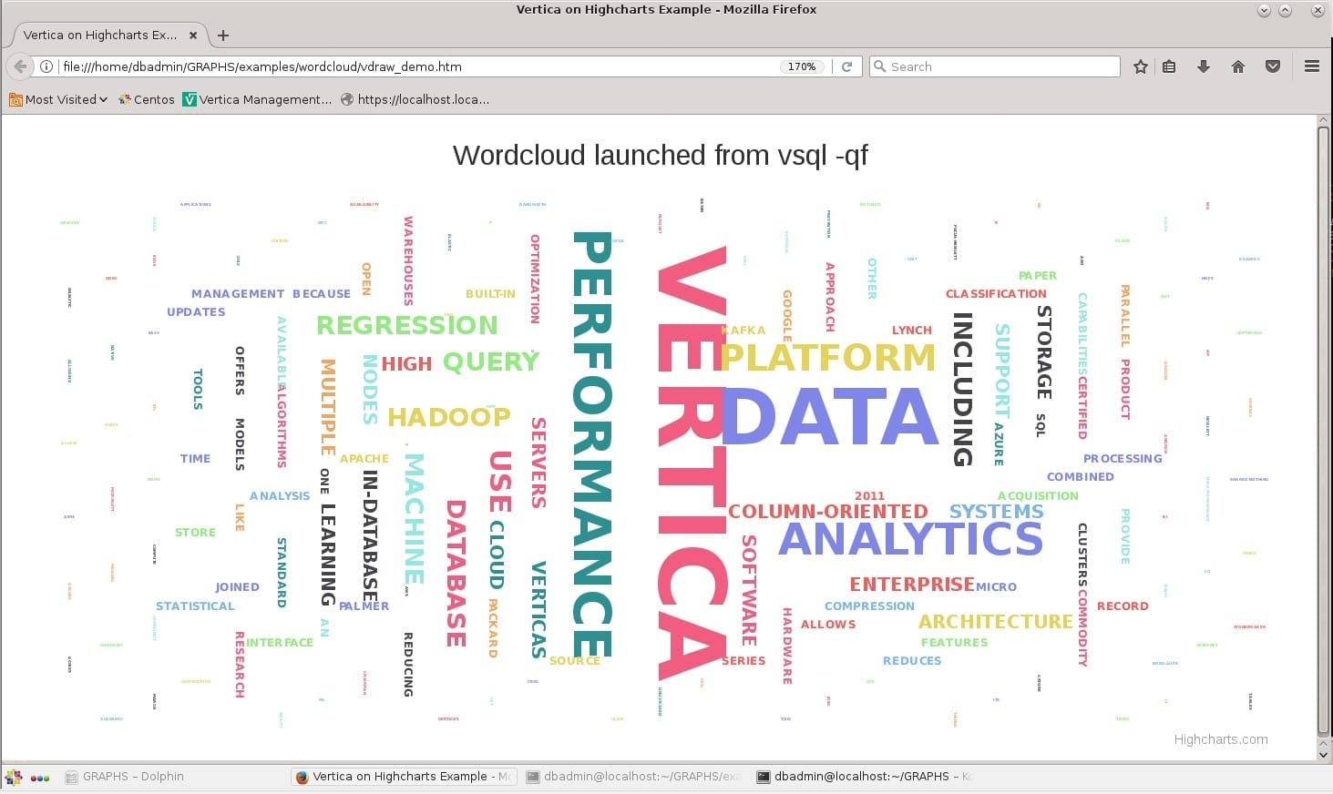
--\q                -- Remove this line after installing highcharts from:  https://www.highcharts.com/download
\pset recordsep ' ' -- specifies the character used to delimit table records (by default a newline)
\o ./examples/wordcloud/vdraw_demo.htm
(SELECT 'var text = ''')
UNION ALL
(SELECT UPPER(TRIM(BOTH ' `~.,-[      ]()’' FROM word)) AS word
FROM vdraw_big_text_table
WHERE UPPER(TRIM(BOTH ' `~.,-[      ]()’' FROM word)) not in ('AND','THE','OF','TO','IN','A','WITH','FOR','ON','AS','WAS','BY','SUCH','AT',
'IS','WHICH','ARE','ALSO'))
UNION ALL
(SELECT ''';');
\o
\pset recordsep '\n' -- specifies the character used to delimit table records (by default a newline)
\! tail -91 ./vdraw.sql | head -22 | cat - ./examples/wordcloud/vdraw_demo.htm > vdraw_temp_file && mv vdraw_temp_file ./examples/wordcloud/vdraw_demo.htm
\! tail -66 ./vdraw.sql | head -31 >> ./examples/wordcloud/vdraw_demo.htm
\! (cd ./examples/wordcloud ; firefox vdraw_demo.htm)
< head>
< meta http-equiv="refresh" content="3">
< /head>
Disclaimer
This document content is for informational purposes only. The content here should not be relied upon as an advice how to run SQL code. Neither Vertica nor Microfocus make any warranties, express, implied, or statutory, as to the information in this document and/or to the provided code. The content here and the SQL Demo provided “as-is.” The information here, including opinions expressed, as well as URLs and other references, may change without notice. This document does not provide any legal rights to any intellectual property contained herein and does not provide any legal rights to use any Microfocus or Vertica product.
About the Author
Moshe Goldberg
Vertica System Engineer
With more than twenty years of experience, in technical consulting, teaching, project management and IT management, today as part of the EMEA SE team I’m happy to work with Vertica as the best product, in a great company, thanks to the unique people here.